6. Running the Code
Carol: Well, let's see what happens. I don't want to look at a thousand
lines of output. I will first run the code, redirecting the results into
an output file, called euler_try.out:
Erica: I agree, we should do that soon. But hey, the numbers do tell us
something already, they tell us that there is something seriously wrong!
Carol: How can you tell?
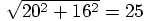
Erica: At the end of the run, the distance between the two particles
is more than 25 in our units, as you can see by applying Pythagoras to the
last numbers in the first two columns:
Dan: So what?
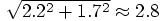
Erica: A bit large already for my taste, but what clinches it is the
velocity difference between the particles, which is more than
Dan: So what?
Erica:
We started out with a velocity difference of only 0.5, so we have
increased the velocity by more than a factor of more than 5, while
increasing the distance by a factor of more than 25. When two
particles move away from each other, they should slow down, not speed
up, because gravity is an attractive force.
Carol: I see, yes, that is strange.
Dan: Even more reason to make a plot!
Carol: How about using gnuplot? That one is present on any
system running Linux, and something that can be easily installed on many
other systems as well. The style is not particularly pretty, but at
least it will give us something to look at.
Dan: How do you invoke gnuplot?
Carol: To use it is quite simple, with only one command
needed to plot a graph. In our case, however, I'll start with the
command set size ratio -1. A positive value for the size
ratio scales the aspect ratio of the vertical and horizontal edge of
the box in which a figure appears. But in our case we want to
set the scales so that the unit has the same length on both the x and
y axes. Gnuplot can be instructed to do so by specifying the ratio to
be -1. In fact, you can write the line set size ratio
-1 in a file called .gnuplot in your home directory, if
you want to avoid repeating yourself each time you use gnuplot.
But for starters, I'll give the command specifically.
The next command we need to use is plot
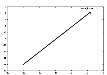
Now let's have our picture, in fig 17:
Figure 17: First attempt at integrating the two-body problem: failure.
Dan: Hmmm, that is not what I expected to see. What a disappointment!
Erica: Well, research is like that -- the first time you do something,
it almost never works.
Carol: Good thing you called the program euler_try.rb!
Dan: It seems as if the system exploded. Why would the two particles
fly apart like that?
Erica: That's what we have to find out. And we'd better be systematic.
Dan: How will we ever find out what is the case? Shall we look at the
code, line by line, to see whether we made a mistake? It is such a short
code, there are not that many ways to do something wrong!
Carol: That's not the right approach. If you are starting from the
wrong assumptions, just looking at the code will not help you to realize
what was wrong with your thinking, no matter how long you stare at it.
Dan: Research is difficult! If this would be an exercise out
of a book, at least the answer would be in the back, or we could ask a
teaching assistant . . .
Erica: Yes, research is difficult, but it also is a lot more fun than
chewing on home work assignments. You know, when you start playing
in your own way, very soon you start doing things that in that exact
form nobody else has ever done before. Isn't that a thrill?!
Dan: It would be a thrill if we could make progress. Frankly, I'm lost.
Carol: I must admit, I don't see a clear way ahead either, but at least
I remember that one of my teachers told us to `divide and conquer' while
troubleshooting. In other words, if something goes wrong in a complex
situation, try to simplify everything by dividing whatever procedure you
have applied in smaller, more modular steps. That way, you can try to
see in which step something goes wrong.
Erica: That makes sense. And I remember hearing a graduate student
tell us, while we were struggling with a computer program: `simplify,
simplify.' The idea was to first look at the simplest possible parameter
choice, because in simpler cases it is often easier to see what goes wrong.
Dan: You mean that we have done too much, too soon, by taking a rather
arbitrary choice of initial conditions, and a thousand steps?
Erica: Exactly. The notion of `divide and conquer' tells us that we'd
better do one integration step at a time, instead of a thousand. And the
idea of `simplify, simplify' suggests that we start with a circular orbit,
rather than the more general case of an elliptic orbit.
Carol: So we have to find out what the correct velocity is, for two
particles at a distance of 1, in order to move in a circle. It seems
to be larger than 0.5, but how much larger?
Dan: Large enough that the particles don't fall toward each other but
not so large that they start moving away from each other. Hmm. How can
we picture that? Imagine that we would move the two particles in a
circular orbit around each other, and measure how much force we have
to use to keep them in the circular orbit. We could then require
gravity to do the work for us, and insist that the gravitational force
would be just equal to the force that we would have to apply by hand.
Erica: Or rather that letting gravity provide the right force,
it is easier to compare accelerations, rather than forces. Let
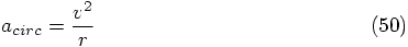
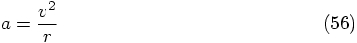
us insist on gravity providing the right acceleration.
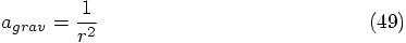
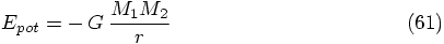
For the equivalent one-body problem, in our choice of units, the
the gravitational acceleration is given in Eq. (42).
Since we are only interested in the magnitude, we can write it as:
Erica: Oh, I just remember, it is one of the standard equations
I learned in classical mechanics.
Dan: Well, I don't remember, and while I'm sort-of happy to take your
word for it, I would be much happier to see whether we can derive it,
so that we know for sure we have the right expression.
Carol: Me too, I'm with Dan here.
Erica: Well, hmmm, I suppose we can go to the library and look it up
in a text book on classical mechanics. Any textbook should tell you how
to derive that expression. Frankly, I don't remember now how we did it.
Dan: It would be much faster to look it up on Google. But of course,
then you have to wonder whether it was done correctly or not.
Carol: Come on, it can't be that hard. And it is much more fun
to derive it ourselves rather than look it up. No Dan, I don't even want
to look at Google. Here, let's take a piece of paper, and derive both the
first and the second derivatives of the scalar distance
Dan: Well, before I ask what you mean, let me first see what you do.
Carol: We start with the definition of
Erica: That makes sense: on a circular orbit the velocity has no
component in the direction toward the other particle, so it is indeed
perpendicular.
Dan: There is something I don't understand. In the equation above,
you start with the expression
Carol: Which they don't. You are confused with the expression
Carol: Until you get used to it.
Dan: Well, that's true for everything.
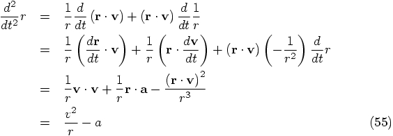
Carol: Fair enough. Okay, onward to the second derivative of the
separation between the two particles:
For a circular orbit, we must insist that the separation
Erica: Neat! Satisfied, Dan?
Dan: Sure thing!
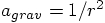
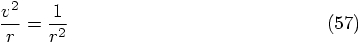
Carol: Let's see why we did all this. Ah, we wanted to balance the
gravitational acceleration provided and the acceleration needed to keep
a motion being nicely circular. We already found that
Dan: Ah, so we should have used
Erica: You know, while Carol was doing her virtuoso derivation act,
I suddenly remembered that there is a much quicker way to derive the
same result from scratch.
Carol: Show me! I find that hard to believe.
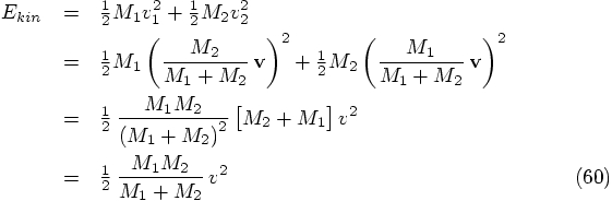
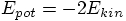
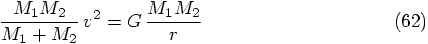
Erica: It just occurred to me that I could use the virial theorem,
which tells us that for any bound system, on average the potential
energy is equal to minus twice the kinetic energy in the c.o.m. frame.
For a circular orbit, both the potential and kinetic energy remain
constant, so we don't even have to do any averaging.
In our case, we can use Eqs. (22) and (24) to write the
kinetic energy as:
Carol: I must admit, you got the right answer and your derivation
is a bit simpler than the one I just gave. But I have never heard of the
virial theorem. What does it mean?
Erica: Weeeeellll, that's quite a long story. I'm not sure whether
we should go into that right now. If you really want to know, you can
look at a text book, but . . .
Dan: . . . Google gives me a whole bunch of sites. Let's look at a few.
Hmmmm. A bit too much math, this one. . . Ah, this one looks easier,
with more words and simple examples . . .
Carol: So we know we can look it up when we have to. I agree with Erica,
I'd rather move on.
Dan: Wait a minute, each of you have just given a detailed derivation,
and now you're suddenly in a hurry. You know what? I bet that I can give
an even simpler derivation, and that without using complicated vector
calculus or the vitrial theorem.
Erica: virial theorem.
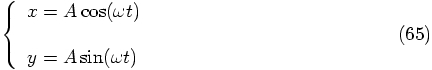
Dan: Whatever. Here is my suggestion. Why not just write down the
circular orbit itself, as if we had already derived it? I don't remember
much from my introductory physics class, but I do remember how neat it
was that you could write down a simple circular motion in two dimensions
in the following way, for the position:
Erica: Yes, it is very simple, I'm surprised!
Dan: I must admit that I'm a bit surprised too, that it came out
so easily. And, frankly, I'm surprised that I came out correctly!
Carol: But working in coordinates like that is not very elegant.
Erica: Oh, come on, Carol, give the guy a break! What counts is
to get the right answer, and you must admit that his solution is
simpler than either of our ways of deriving the same answer. Let's
just be glad that all three methods gave the same answer!
Carol: Ah, you physicists, you're so pragmatic! I'd prefer a bit
more style.
Dan: Well, each her own style. I'm happy now, and ready to move on!
Erica: Which means that we've answered the `simplify, simplify'
part of our task of trouble shooting: we now know how to launch the
two-body problem on the simplest possible orbit, that of a circle.
The other task was `divide and conquer', and we had already decided
to start with just one step.
Dan: That's a simple change in our program: we can just take out the
loop.
Carol: Okay, here is the new code. Let me call it
euler_try_circular_step.rb.
Dan: You sure like long names! I would have called it
euler_trycs.rb.
Carol: Right. And three days later you will be wondering why there
is a program floating around in your directory that seems to tell you
that it uses Euler's algorithm for trying out cool stuff, or for
experimenting with communist socialism or for engaging in some casual sin.
No, I'm a big believer in looooong names.
Erica: I used to be like Dan, but I've been bitten too often by the
problem you just mentioned, that I could for the life of me not remember
what the acronym was supposed to mean that I had introduced. So yes,
I'm with you.
Dan: Fine, two against one, I lose again! But I'll be gs, oops,
I mean a good_sport.
Carol: What do you think of this version
of euler_try_circular_step.rb?
Erica: Let's see: you got the circular velocity correct,
a value of unity as it should be. And instead of looping,
you print, take one step, and print again. Hard to argue with!
Dan: Let's see whether it gives a reasonable result. 6.1. A Surprise
|gravity> ruby euler_try.rb > euler_try.out
In that way, we can look at our leisure at the beginning and at the
end of the output file, while skipping the 991 lines in between
times 0, 0.01, 0.02, 0.03, 0.04 . . . 9.96, 9.97, 9.98, 9.99, 10.
 |gravity> head -5 euler_try.out
 1  0  0  0  0.5  0
 1.0  0.005  0.0  -0.01  0.49  0.0
 0.9999  0.0099  0.0  -0.0199996250117184  0.480000374988282  0.0
 0.999700003749883  0.0147000037498828  0.0  -0.0300001547537506  0.469999845246249  0.0
 0.999400002202345  0.0194000022023453  0.0  -0.0400029130125063  0.459997086987494  0.0
 |gravity> tail -5 euler_try.out
 -19.9935403671885  -16.0135403671885  0.0  -2.24436240147761  -1.74436240147762  0.0
 -20.0159839912033  -16.0309839912033  0.0  -2.24435050659793  -1.74435050659793  0.0
 -20.0384274962693  -16.0484274962693  0.0  -2.24433863791641  -1.74433863791641  0.0
 -20.0608708826484  -16.0658708826485  0.0  -2.24432679534644  -1.74432679534644  0.0
 -20.0833141506019  -16.0833141506019  0.0  -2.2443149788018  -1.74431497880181  0.0
Dan: A lot of numbers. Now what? We'd better make a picture of the
results, to see whether these numbers make sense or not. Let's plot the
orbit.
 .
.
 .
.
 |gravity> gnuplot
 gnuplot> set size ratio -1
 gnuplot> plot "euler_try.out"
 gnuplot> quit
6.2. Too Much, Too Soon
6.3. A Circular Orbit
 between the two particles. When we force both derivatives to be zero,
we now that
between the two particles. When we force both derivatives to be zero,
we now that  will remain constant forever, since
equations of motion are second-order differential equations.
will remain constant forever, since
equations of motion are second-order differential equations.
6.4. Radial Acceleration
 as the absolute
value or, if you like, the length of the vector
as the absolute
value or, if you like, the length of the vector  :
:


 , and the only way
to guarantee this, according to the equation I just derived, is to
insist that the vectors
, and the only way
to guarantee this, according to the equation I just derived, is to
insist that the vectors  and
and  are
perpendicular, so that
are
perpendicular, so that  .
.
 . But isn't that the
velocity? If you insist that
. But isn't that the
velocity? If you insist that  , aren't you telling
us that the velocity is zero? But in that case the two particles would
start falling toward each other, the next moment!
, aren't you telling
us that the velocity is zero? But in that case the two particles would
start falling toward each other, the next moment!
 which is the absolute value of the velocity,
and it is a very different beast than what I just wrote down. So it
is important to realize that, yes, in a one-dimensional situation you
can write
which is the absolute value of the velocity,
and it is a very different beast than what I just wrote down. So it
is important to realize that, yes, in a one-dimensional situation you
can write

 points in the opposite direction
of the separation vector
points in the opposite direction
of the separation vector  , which means that
 .
.
 between the particles remains constant.
This means that the time derivative
between the particles remains constant.
This means that the time derivative  ,
and of course the same holds for the second derivative in time,
,
and of course the same holds for the second derivative in time,
 . And there we are, Eq. (55) then
gives us:
. And there we are, Eq. (55) then
gives us:
 , so this means:
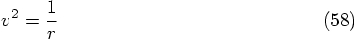

 which implies
  ,
but we used an initial velocity of
,
but we used an initial velocity of  which
means that
which
means that  , much too small a value for a circular
orbit! It should have been
, much too small a value for a circular
orbit! It should have been  , according to what we just
derived.
, according to what we just
derived.
 for the
initial velocity. Great! Good to know.
for the
initial velocity. Great! Good to know.
6.5. Virial Theorem
 ,
which gives us:
,
which gives us:
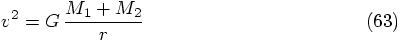
 and therefore we have:
6.6. Circular Motion
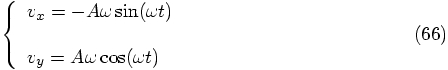

 we have
  , so this means that
 . Well, Eq. (66) now tells us
that
. Well, Eq. (66) now tells us
that  . Isn't that simple?
6.7. One Step at a Time