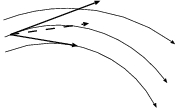
10. The Modified Euler Algorithm
Dan: Well, Erica, how are we going to move up to a more accurate
algorithm?
Carol: You mentioned something about a second-order scheme.
Erica: Yes, and there are several different choices. With our
first-order approach, we had little choice. Forward Euler was the
obvious one: just follow your nose, the way it is pointed at the
beginning of the step, as in fig. 15.
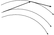
Dan: You mentioned a backward Euler as well, and even drew a picture,
in in fig. 16.
Erica: That was only because you asked me about it! And the backward
Euler scheme is not an explicit method. It is an implicit method, where
you have to know the answer before give calculate it. As we discussed, you
can solve that through iteration; but in that case you have to redo every
step at least one more time, so you spend a lot more computer time and
you still only have a first-order method, so there is really no good reason
to use that method.
Carol: But wait a minute, the two types of errors in figs. 15
and 16 are clearly going in the opposite directions.
I mean, forward flies out of the curve one way, and backward spirals in
the other way. I wonder, can't you somehow combine the two methods and
see whether we can let the two errors cancel each other?
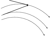
If we combine the previous two pictures, the most natural thing would be
to try both of the Euler types, forward and backward. Here is a sketch,
in fig. 29. The top arrow is what we've done so far,
forward Euler, simply following the tangent line of the curve. The
bottom line is backward Euler, taking a step that lands on a curve
with the right tangent at the end. My idea is to compute both, and then
take the average between the two attempts. I'm sure that would give a
better approximation!
Figure 29: An attempt to improve the Euler methods. The top arrow shows forward Euler,
and the bottom arrow backward Euler. The dashed arrow shows the average
between the two, which clearly gives a better approximation to the curved
lines that show the true solutions to the differential equation.
Carol: It was just a wild idea, and it may not be useful.
Erica: Actually, I like Carol's idea. In reminds me of one of the second
order schemes that I learned in class. Let me just check my notes.
Aha, I found it. There is an algorithm called "Modified Euler", which
starts with the forward Euler idea, and then modifies it to improve the
accuracy, from first order to second order. And it seems rather similar
to what Carol just sketched.
Carol: In that case, how about trying to reconstruct it for ourselves.
That is more fun than copying the algorithm from a book.
Now let's see. We want to compute the dashed line in figure 29.
How about shifting the arrow of the backward step to the end
of the arrow of the forward step, as in fig. 30? Or to be
precise, how about just taking two forward Euler steps, one after the other?
The second forward step will not produce exactly the same arrow as the first
backward step, but it will be almost the same arrow, and perhaps such an
approximation would be good enough.
Figure 30: Two successive forward Euler steps.
Carol: How about shifting the second arrow back, in fig. 30,
so that the end of the arrow falls on the same point as the end of the
first arrow? In that way, we have constructed a backward Euler step
that lands on the same point where our forward Euler step landed, as
you can see in fig. 31.
Figure 31: A forward Euler steps and a backward Euler step, landing at the same point.
10.1. A Wild Idea
10.2. Backward and Forward
The simplest way to construct the average between the two vectors is by adding them and then dividing the length by two. Here it is, in fig. 32.
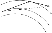
Figure 32: The new integration scheme produces the dashed arrow, as exactly one-half of the some of the two fully drawn arrows; the dotted arrow has the same length as the dashed arrow. This result is approximately the same as the dashed arrow in fig. 29.
10.3. On Shaky Ground
Dan: I don't believe it. Or what I really mean is: I cannot yet believe that this is really correct, because I don't see any proof for it. You are waving your arms and you just hope for the best. Let's be a bit more critical here.
In figure 29, it was still quite plausible that the dashed arrow succeeded in canceling the opposite errors in the two solid arrows. Given that those two solid arrows, corresponding to forward Euler and backward Euler, were only first-order accurate, I can see that the error in the dashed arrow just may be second-order accurate. Whether the two first-order errors of the solid arrows actually cancel in leading order, I'm not sure, but we might be lucky.
But then you start introducing other assumptions: that you can swap the new second forward Euler arrow for the old backward Euler error, and stuff like that. I must say, here I have totally lost my intuition.
Frankly, I feel on really shaky ground, talking about an order of a differential equation. I have some vague sense of what it could mean, but I wouldn't be able to define it.
Erica: Here is the basic idea. If an algorithm is nth order, this means that it makes an error per step that is one order higher in terms of powers of the time step. What I mean is this: for a simple differential equation
 to time
  , with
  ,
can be written as:
,
can be written as:

 is a function of
 , but it is almost independent of the size of the time
step
, but it is almost independent of the size of the time
step  , and in the limit that
  , it will converge to a constant value
 , which in the general case will
be proportional to the (n+1) th time derivative of
, which in the general case will
be proportional to the (n+1) th time derivative of
 , along the orbit
  .
.
In practice, we want to integrate an orbit over a given finite interval
of time, for example from  to
to
 . For a choice of step size
  , we then
need
, we then
need  integration steps. If we assume that the
errors simply add up, in other words, if we don't rely on the errors
to cancel each other in some way, then the total integration error
after
integration steps. If we assume that the
errors simply add up, in other words, if we don't rely on the errors
to cancel each other in some way, then the total integration error
after  steps will be bounded by

 is proportional to an upper bound of the absolute
value of the (n+1) th time derivative of
is proportional to an upper bound of the absolute
value of the (n+1) th time derivative of  ,
along the orbit
,
along the orbit  .
.
In other words, for an nth order algorithm, the error we make
after integrating for a single time step scales like the
(n+1) th power of the time step, and the error we make after
integrating for a
Dan: I'm now totally confused. I don't see at all how these higher derivatives of f come in. In any case, for the time being, I would prefer to do, rather than think too much. Let's just code up and run the algorithm, and check whether it is really second order.
Erica: That's fine, and I agree, we shouldn't try to get into a complete numerical analysis course. However, I think I can see what Carol is getting at. If we apply her reasoning to the forward Euler algorithm, which is a first order algorithm, we find that the accumulated error over a fixed time interval scales like the first power of time. Yes, that makes sense: when we have made the time step ten times smaller, for example in sections 7.3 and 8.2, we have found that the error became roughly ten times smaller.
Carol: So if the modified Euler algorithm is really a second-order algorithm, we should be able to reduce the error by a factor one hundred, when we make the time step ten times smaller.
Erica: Yes, that's the idea, and that would be great! Let's write a code for it, so that we can try it out.
Dan: I'm all for writing code! Later we can always go back to see what the theory says. For me, at least, theory makes much more sense after I see at least one working application.
Carol: It should be easy to implement this new modified Euler scheme.
The picture we have drawn shows the change in position of a particle, and we
should apply the same idea to the change in velocity.
For starters, let us just look at the position. First we have to
introduce some notation.
Erica: In the literature, people often talk about predictor-corrector
methods. The idea is that you first make a rough prediction about a
future position, and then you make a correction, after you have
evaluated the forces at that predicted position.
In our case, in fig. 32, the first solid arrow starts at
the original point
Erica: I know, we'll come to that in a moment, when we write down the
velocity equivalent for Eq. (81). I just wanted to write
the position part first. We can find the corrected new position by
taking the average of the first two forward Euler steps, as indicated
in fig. 32:
Erica: Yes, in fact it is just a matter of differentiating the previous
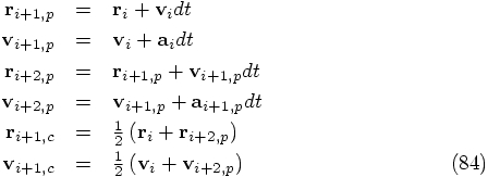
lines with respect to time. Putting it all together, we can calculate
all that we need in the following order, from predicted to corrected
quantities:
Carol: Here is the new code.
I'll call it euler_modified_10000_steps_sparse.rb. Let's
hope we have properly modified the original Euler:
Carol:
As you can see I am giving it time steps of size 0.001, just to be on
the safe side. Remember, in the case of plain old forward Euler, when
we chose that step size, we got
figure 24. Presumably, we will
get a more accurate orbit integration this time. Let's try it!
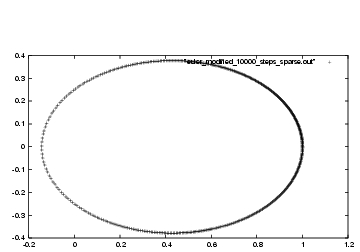
Figure 33: First attempt at modified Euler integration, with step size
Dan: Wow!!! Too good to be true. I can't even see deviations from the
true elliptic orbit! This is just as good as what we got for forward
Euler with a hundred times more work, in figure
26.
Erica: fifty times more work, you mean. In figure
26, we had used time steps of
Dan: Ah, yes, you're right. Well, I certainly don't mind doing twice
as much work per step, if I have to do far fewer than half the number
of steps!
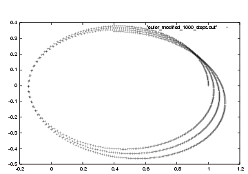
Carol: Let's try to do even less work, to see how quickly things get bad.
Here, I'll make the time step that is ten times larger, in the file
euler_modified_1000_steps.rb. This also makes life a little
simpler, because now we no longer have to sample: we can produce one
output for each step, in order to get our required one thousand outputs:
Carol:
This approach should need just twice as much work as our very first attempt
at integrating the elliptic orbit, which resulted in failure, even
after we had corrected our initial typo, as we could see in figure 22.
Figure 34: Second attempt at modified Euler integration, with step size
Dan: Yes, it seems clear that our modified Euler behaves a lot better
than forward Euler. But we have not yet convinced ourselves that it is
really second order. We'd better test it, to make sure.
Carol: Good idea. Here is a third choice of time step, ten times smaller
than our original choice, in file
euler_modified_100000_steps_sparse.rb:
With the three choices of time step, we can now compare the last output
lines in all three cases:
In other words, if we take the last outcome as being close to the true
result, then the middle result has an error that it about one hundred
times smaller than the first result. The first result has a time step
that is ten times larger than the second result. Therefore, making the
time step ten times smaller gives a result that is about one hundred
times more accurate. We can congratulate ourselves: we have clearly
crafted a second-order integration algorithm! 10.4. Specifying the Steps
 . Let us call the end point of that
arrow
. Let us call the end point of that
arrow  , where the p stands for predicted,
as the predicted result of taking a forward Euler step:
, where the p stands for predicted,
as the predicted result of taking a forward Euler step:

 :
:

 ,
something that you haven't calculated yet.
,
something that you haven't calculated yet.
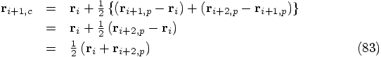
 instead
of
instead
of  and
and  instead of
  .
.
 is calculated just before it is needed in calculating
 , just as Erica correctly predicted
(no pun intended).
, just as Erica correctly predicted
(no pun intended).
10.5. Implementation
10.6. Experimentation
|gravity> ruby euler_modified_10000_steps_sparse.rb > euler_modified_10000_steps_sparse.out
 .
.
 , a hundred times smaller than the time steps of
 that we used in figure 33;
but in our modified Euler case, each step requires twice as much work.
that we used in figure 33;
but in our modified Euler case, each step requires twice as much work.
10.7. Simplification
|gravity> ruby euler_modified_1000_steps.rb > euler_modified_1000_steps.out
 .
.
10.8. Second Order Scaling
 |gravity> ruby euler_modified_1000_steps.rb | tail -1
 0.400020239524913  0.343214474344616  0.0  -1.48390077762002  -0.0155803976141248  0.0

 |gravity> ruby euler_modified_10000_steps_sparse.rb | tail -1
 0.598149603243697  -0.361946726406968  0.0  1.03265486807376  0.21104830479922  0.0

 |gravity> ruby euler_modified_100000_steps_sparse.rb | tail -1
 0.59961042861231  -0.360645741133914  0.0  1.03081178933713  0.213875737743879  0.0
Well, that's pretty clear, isn't it? The difference between the last
two results is about one hundred times smaller, that the difference
between the first two results.