23. Error Behavior for 2nd-Order Schemes
Erica: I want to see how the error accumulates over a few orbits.
We saw in figure 46 how the total energy error
grows monotonically, with energy conservation getting a whack each
time te stars pass close to each other. I wonder whether our two
second-order schemes show a similar behavior, or whether things are
getting more complicated.
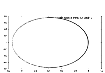
Carol: Easy to do. As before, I will remind us what
the orbit looked like, by plotting the
Figure 47: Trajectory using a modified Euler algorithm.
with
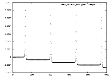
Carol: And here is how the error grows, as a function of time,
in fig 48.
Figure 48: Energy error growth using a modified Euler algorithm.
with
Erica: I think I know what's going on. The original forward Euler
algorithm was making terrible errors at pericenter. I'm sure that the
backward Euler algorithm would be making similarly terrible errors when
the stars pass each other at pericenter. Now the modified Euler scheme
works so well because it almost cancels those two errors.
In other words, during pericenter passage, the errors in forward and
in backward Euler grow enormously, and the attempt at canceling is
relatively less successful. But once we emerge from the close encounter,
the attempts at canceling have paid off, and the net result is a much
more accurate energy conservation.
Carol: Hmm, that sounds too much like a hand-waving argument to me.
I would be more conservative, and just say that second-order
algorithms are more complicated to begin with, so I would expect them
to have more complex error behavior as well. Your particular
explanation may well be right, but can you prove that?
Erica: I'm not sure how to prove it. It is more of a hunch.
Dan: Let's not get too technical here. We want to move stars around,
and we don't need to become full-time numerical analysts.
Erica: But I would like to see what happens when we make the time
step smaller.
Carol: Okay, I'll make the time step ten time smaller, and plot the
results in fig 49.
Figure 49: Energy error growth using a modified Euler algorithm.
with
Erica: But the error peaks scale like a second-order algorithm: they have
become 100 times less high.
Carol: So the net error after the whole run must have scaled better than
second-order. And indeed, look at the output we got when I did the
runs: after ten time units, the energy error became a factor thousand
smaller, when I decreased the time step by a factor ten!
Dan: Almost too good to be true.
Carol: Well, a second-order scheme is guaranteed to be at least second
order; there is no guarantee that it doesn't do better than that. It may
be the particular configuration of the orbit that gives us extra error
cancellation, for free. Who knows?
Dan: Let's move on and see what the leapfrog algorithm shows us.
Carol: Okay. First I'll show the orbit, in
fig 50, using leapfrog_energy.rb:
Figure 50: Trajectory using a leapfrog algorithm.
with
Carol: And here is how the error grows, as a function of time,
in fig 51.
Figure 51: Energy error growth using a leapfrog algorithm.
with
Erica: That makes sense, actually. Remember, the leapfrog is time
symmetric. Imagine that the energy errors increased in one direction
in time. We could then reverse the direction of time after a few orbits,
and we would play the tape backward, returning to our original starting
point. But that would mean that in the backward direction, the energy
errors would decrease. So that would spoil time symmetry: if the
errors were to increase in one direction in time, they should increase
in the other direction as well. The only solution that is really time
symmetric is to let the energy errors remain constant, neither
decreasing nor increasing.
Carol: Apart from roundoff.
Erica: Yes, roundoff is not guaranteed to be time symmetric. But as long
as we stay away from relative errors of the order of
Carol: Time to check what happens for a ten times smaller time step:
Figure 52: Energy error growth using a leapfrog algorithm.
with
Erica: And so is the scaling for the total error at the end of the
whole run: it, too, is a hundred times smaller.
Dan: But wait a minute, you just argued so eloquently that the leapfrog
algorithm should make almost no error, in the long run.
Erica: Yes, either in the long run, or after completing exactly one
orbit -- or any integer number of orbits, for that matter. But in our
case, we haven't done either. After ten time units, we did not return
to the exact same place.
You see, during one orbit, the leapfrog can make all kind of errors.
It is only after one full orbit that time symmetry guarantees that
the total energy neither increases or decreases. And compared to
other algorithms, the leapfrog would do better in the long run, even
if you would not stop after an exact integer number of orbits,
compared to a non-time-symmetric scheme, such as modified Euler. The
latter would just keep building up errors at every orbit, adding the
same systematic contribution each time.
Dan: I'd like to see that. Let's integrate for an exact number of
orbits.
Erica: Good idea. I also like to test the idea, to see how well it
works in practice. But first we have to know how long it takes for
our stars to revolve around each other.
Let's see. In the circular case that we have studied before, while
we were debugging, we started with the following initial conditions,
where I am adding the subscript c for circular:
Dan: Let's bring up a calculator on your screen.
Carol: Why not stay with Ruby and use irb? We can use the fact
that
Erica: Yes, and indeed, if you look at fig. 45,
you can see that our stars have almost completed four orbits by
time
Carol: Let's see whether we can find a good time to stop. Since we
do an output every
Carol: Sure, why not ten times larger:
Carol: Here it is
23.1. Modified Euler: Energy Error Peaks
 coordinates of the position, in fig 47.
 |gravity> ruby euler_modified_energy.rb > euler_modified_energy.out
 time step = ?
 0.001
 final time = ?
 10
   t = 0,   E_kin = 0.125, E_pot = -1; E_tot = -0.875
             E_tot - E_init = 0, (E_tot - E_init) / E_init = -0
   t = 10,   E_kin = 0.555, E_pot = -1.43; E_tot = -0.875
             E_tot - E_init = 0.000118, (E_tot - E_init) / E_init = -0.000135
 .
.
 .
.
23.2. Almost Too Good
 |gravity> ruby euler_modified_energy.rb > euler_modified_energy2.out
 time step = ?
 0.0001
 final time = ?
 10
   t = 0,   E_kin = 0.125, E_pot = -1; E_tot = -0.875
             E_tot - E_init = 0, (E_tot - E_init) / E_init = -0
   t = 10,   E_kin = 0.554, E_pot = -1.43; E_tot = -0.875
             E_tot - E_init = 1.17e-07, (E_tot - E_init) / E_init = -1.34e-07

 .
.
23.3. Leapfrog: Peaks on Top of a Flat Valley
 |gravity> ruby leapfrog_energy.rb > leapfrog_energy.out
 time step = ?
 0.001
 final time = ?
 10
   t = 0,   E_kin = 0.125, E_pot = -1; E_tot = -0.875
             E_tot - E_init = 0, (E_tot - E_init) / E_init = -0
   t = 10,   E_kin = 0.554, E_pot = -1.43; E_tot = -0.875
             E_tot - E_init = 3.2e-07, (E_tot - E_init) / E_init = -3.65e-07

 .
.

 .
.
 ,
what I said should hold accurately. This most be the explanation for
the fact that the baseline errors in fig 51, in
between the periastron peaks, remain so level.
,
what I said should hold accurately. This most be the explanation for
the fact that the baseline errors in fig 51, in
between the periastron peaks, remain so level.
 |gravity> ruby leapfrog_energy.rb > leapfrog_energy2.out
 time step = ?
 0.0001
 final time = ?
 10
   t = 0,   E_kin = 0.125, E_pot = -1; E_tot = -0.875
             E_tot - E_init = 0, (E_tot - E_init) / E_init = -0
   t = 10,   E_kin = 0.554, E_pot = -1.43; E_tot = -0.875
             E_tot - E_init = 3.2e-09, (E_tot - E_init) / E_init = -3.65e-09

 .
.
23.4. Time Symmetry


 .
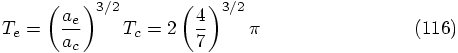
The orbital period, the time to go around the whole orbit, is therefore:
.
The orbital period, the time to go around the whole orbit, is therefore:


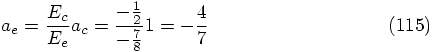
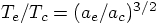
 of a Kepler orbit
is inversely proportional to the total energy, we can use the
results from the circular orbit to find the semi-major axis
for our eccentric orbit:
of a Kepler orbit
is inversely proportional to the total energy, we can use the
results from the circular orbit to find the semi-major axis
for our eccentric orbit:
 , or:
, or:
23.5. Surprisingly High Accuracy
 :
:
 |gravity> irb
 include Math
 Object
 pi = 2*acos(0)
 3.14159265358979
 t = (4.0/7.0)**1.5 * 2 * pi
 2.7140809410828
 quit
Dan: Ah, so four orbits would be close to our total integration time
of ten time units, but just a bit longer.
 , but not quite yet.
 , it would be nice to
find an integer number of orbits that would also be close to a multiple
of
, it would be nice to
find an integer number of orbits that would also be close to a multiple
of  , so that we can end the integration at that
time. I'll try a few values:
, so that we can end the integration at that
time. I'll try a few values:
 |gravity> irb
 include Math
 Object
 pi = 2*acos(0)
 3.14159265358979
 t = (4.0/7.0)**1.5 * 2 * pi
 2.7140809410828
 4 * t
 10.8563237643312
 6 * t
 16.2844856464968
 7 * t
 18.9985665875796
 quit
Ah, seven orbits brings us very close to  .
Okay, let me integrate for 19 time units:
.
Okay, let me integrate for 19 time units:
 |gravity> ruby leapfrog_energy.rb > /dev/null
 time step = ?
 0.001
 final time = ?
 19
   t = 0,   E_kin = 0.125, E_pot = -1; E_tot = -0.875
             E_tot - E_init = 0, (E_tot - E_init) / E_init = -0
   t = 19,   E_kin = 0.125, E_pot = -1; E_tot = -0.875
             E_tot - E_init = 2.5e-13, (E_tot - E_init) / E_init = -2.85e-13
Erica: That's an amazing accuracy, for such a large time step!
Can you try an even larger time step?
 |gravity> ruby leapfrog_energy.rb > /dev/null
 time step = ?
 0.01
 final time = ?
 19
   t = 0,   E_kin = 0.125, E_pot = -1; E_tot = -0.875
             E_tot - E_init = 0, (E_tot - E_init) / E_init = -0
   t = 19,   E_kin = 0.125, E_pot = -1; E_tot = -0.875
             E_tot - E_init = 1.02e-10, (E_tot - E_init) / E_init = -1.17e-10
Erica: Still a very good result. Remind me, what did we get when we
did our shorter standard integration of ten time units?
 |gravity> ruby leapfrog_energy.rb > /dev/null
 time step = ?
 0.01
 final time = ?
 10
   t = 0,   E_kin = 0.125, E_pot = -1; E_tot = -0.875
             E_tot - E_init = 0, (E_tot - E_init) / E_init = -0
   t = 10,   E_kin = 0.553, E_pot = -1.43; E_tot = -0.875
             E_tot - E_init = 3.18e-05, (E_tot - E_init) / E_init = -3.63e-05
And indeed a lot worse than integrating for 19 time units. I begin
to see the strength of time symmetric integration schemes! Many orders
of magnitude gain in final accuracy, as long as you return to the same
location in the orbit that you started from!
 . Here is one:
201 orbits will take a total time
. Here is one:
201 orbits will take a total time  ,
close to
,
close to  . That should be good enough. Here goes: