1. First-Order Differential Equations
Bob: It has been a lot of fun, to derive so many different algorithms
and to implement them all in our two-body code.
Alice: Yes, I enjoyed it too, and I must admit, I learned a lot in the
process. But I still have the feeling that I'm missing some basic pieces
of insight. Do you remember how we struggled, trying to prove that the
Abramowicz and Stegun formula was correct, the fourth-order
Bob: But you figured it out, didn't you?
Alice: Well, yes, after a false start. And it was a bit alarming that
at first I didn't even realize that it was a false start. And to be
completely honest, even now I'm not a full hundred percent sure that
we got things right. Let me put it this way, I feel that I haven't
yet gotten a finger-tip feeling for what Runge-Kutta schemes are, and
how they really tick.
Bob: There must be several text books that you can look at. Surely they
will explain things in more depth than you want to know.
Alice: I did look at some books on numerical methods, but none of them
gave me what I really wanted to see. Some of them were just too
mathematical in their concern and notation, others didn't provide the
type of real detail that I wanted to see, yet others specialized on
particular approaches. What I really would like to see is a pedestrian
approach, no attempt to design special improvements. While I'm interested
in all the extras, from embedded higher-order schemes to using extrapolation
methods and symplectic schemes and what have you, I really would like to
first understand the basics better.
Bob: You mean, just the straightforward Runge-Kutta schemes of relatively
low order, without any extra bells and whistles?
Alice: Exactly. Here is an idea. If we limit ourselves to performing
at most two new force calculations per time step, things can't possibly
get too complex. Our Abramowicz and Stegun formula already had three
force calculations per time step, and I'm not suggesting that we explore
explicitly the whole landscape around that formula, at least not yet.
Bob: So you want to explore a smaller landscape, just to see in front of
your eyes how everything works. And while the simplest schemes, like
forward Euler and leapfrog, use only one new force calculation per
time step, you want to explore the full landscape of two new force
calculations per time step. Hmm, I like that. And I'm sure it would
be good for our students too, to see such an explicit survey.
Alice: I think so, but really, right now my main motivation is just for
myself to see exactly how those classical Runge-Kutta derivations are done,
from scratch, without taking anything on faith.
Bob: I like the idea, and I'm game. Where shall we start?
Alice: One problem for astronomers using books on numerical solutions
to differential equations is that most books focus on first-order
differential equations. In contrast, we typically work with
second-order differential equations, and often ones with special
properties. The gravitational equations of motion for the N-body
problem, for example, have a force term that is independent of time
and velocity.
This suggests to me that we should divide our work into two stages.
First we try to figure out how to solve a general first-order
differential equation, using up to two force calculations per step.
This will reproduce the results from the standard text books, no
doubt, but it will give us experience and will allow us to establish
a notation and a systematic procedure.
Then, in the second stage, we can cut our teeth on the gravitational
N-body system, to see what special methods will work there, and why,
and how. The Abramowicz and Stegun formula, for example, is tailored
already to second-order differential equations, albeit a general one
in which there is still a possible velocity dependence present in the
force calculations. We can go one step further, specializing to
position dependence only, and just see what spectrum of methods we
will find.
Then, with a bit of luck, we will have gained enough experience to be
able to look over the horizon, to get an idea what you could do with,
say, three new force calculations per step, which is the landscape
within which the Abramowicz and Stegun formula was grown.
Bob: A somewhat ambitious project, but still quite doable, I think.
You basically want to take the next step beyond forward Euler and
leapfrog, in any possible direction, and see the dimensionality of the
space of possible directions.
Alice: Something like that, yes. But let us restrict ourselves,
at least at first, to Runge-Kutta methods. This will mean no multi-step
methods, such as the original Aarseth scheme. It also means that we
won't use higher derivatives, such as the Hermite scheme. In addition,
we will exclude the use of implicit methods, which require iteration.
Bob: You could argue that, with two new force calculations per time step,
you should allow implicit schemes that have just one new force calcuation
per time step.
Alice: You could, even though it is not immediately clear that one iteration
will provide you sufficiently rapid convergence. Also, the resulting class of
implicit schemes is rather restricted. Perhaps we can look at that later.
For now, I really want to be austere and stay to the absolute basics.
Bob: Okay: explicit Runge-Kutta methods using up to two new force
calculations per time step, and no evaluations of jerks or anything else.
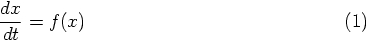
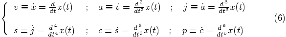
Alice: Let us start by choosing a specific notation.
For the simplest form of differential equation, we can write:
Bob: Even though this is just a warming-up exercise, it would be nice to
give a physical interpretation to the first-order differential equation
that you wrote down:
Alice: In principle that is correct, but in practice, if we have a lot of
resistance, it is the velocity that is proportional to the force. If you
move a spoon through molasses, you have to push twice as hard to go twice
as fast.
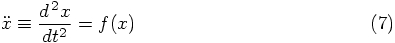
Bob: But even in that case, the initial acceleration must still be
proportional to the applied force.
Alice: Yes, but only very briefly. As soon as you pick up a very small
amount of speed, friction starts to resist, canceling part of your force.
So after the initial transients die out, the velocity settles to a constant
value, proportional to the force you use. From than on, in the limit
of changes that are slow with respect to the duration of the transients,
the acceleration is proportional to the rate of change of the force,
not to the magnitude of the force.
Bob: I don't like the idea of posing a problem, and then neglecting the
interesting part of the solution, namely the transients.
Alice: So for once you are looking for a more clearly abstract model;
I thought you would like a quick and dirty physics example!
Bob: Molasses may indeed be too dirty for me. Why don't we stick with
considering
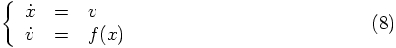
Alice: But the left hand side of the differential equation is a velocity.
The right-hand side has to be something else. In Newtonian dynamics
we have
Bob: Well, yeah, hmmm, let's see, that's not so clear.
Alice: Forgive the pun, but why don't we stick to molasses?
Bob: Ah, I got it! Hey, elementary, my dear Watson.
If a particle would be rolling down a potential well, without
any friction, the total energy would be constant. If we write
Bob: Okay, so we're talking now about a particle in a potential well.
Alice: You may, but I still prefer to talk about molasses, since in
that case we can make a more smooth transition to the case of a second
order differential equation.
Bob: I still prefer my interpretation. Let's just agree to disagree.
Alice: Fine with me, since, after all, the math will be the same.
Bob: Exactly. Okay, let's get to work. You have struggled with these
things a lot more than I have. How do we get started?
Alice: We want to check the quality of any given numerical approximation
scheme to the solution of our differential equation. In order to do
so, we can compare such a scheme with a Taylor series development of
the true solution, around the starting point of our one integration
step.
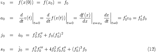
In other words, we can express the position at the end of one time step
in the following Taylor series:
By the way, here the acceleration comes out nicely as the rate
of change of the force applied, as would happen for a spoon moving
slowly through molasses.
Bob: That would take a lot of getting used to! For me, the acceleration
is just the rate of change of the velocity.
Alice: But isn't that a tautology? After all, the acceleration is
by definition the rate of change of the velocity, as a mathematical
construction. I thought we were trying to come up with a physical system
as an example.
Bob: But a potential well is surely a physical system! And what I thought
is that we had agreed to disagree.
Alice: I agree!
Bob: Me too. Coming back to our task,
I like the systematic approach idea, of using up to two
new force evaluations per time step. Well, this gives us two
choices: either one or two force evaluations.
Alice: Actually, there are four choices. In each case, we can try
to recycle a previous force calculation in the next step, or we don't.
Bob: You mean that you use the last force calculation, at the end of
a given step, as the first force value that you use for the next step?
Alice: Exactly. And this will put rather strict conditions on the
nature of that force calculation.
Bob: It means, of course, that a force calculation needs to take place
at the boundary of two steps, otherwise you can't recycle it. But that
doesn't seem to be a particularly severe restriction to me.
Alice: In principle, you could even recycle a force that is used in the
middle, if you would be willing to used the remembered values of the
previous step, you could still recycle. However, that would mean that
we would go beyond Runge-Kutta methods, and enter the area of multi-step
methods.
Bob: Let's not get into that, at least not know. I'd be happy to first
explore the landscape of Runge-Kutta algorithms. Okay, as long as we let
our last force calculation occur at the end of a step, we can recycle that
calculation for the next step.
Alice: Oh, no, it's not that simple. In a general Runge-Kutta approach,
you compute a few forces here and there, and only after doing that, you
combine those forces in such a way as to get a combination of them,
to give you a value of the new position accurate to high order.
Now the force that you would evaluate at that new position, at the
beginning of the next time step, will in general not be the same as
the force that you have calculated at the end of the current time step.
Even though it was evaluated at the same time, it will in general be
evaluated at a slightly different place. The reason is that at the
time of evaluation, you didn't yet have in hand the most accurate
estimate for the new position.
Bob: Hmm, that's tricky. I hadn't thought about that.
Alice: I hadn't either, until I started playing with some of those
schemes in detail. All the more reason to take a really pedestrian
approach, and just write everything out, to make sure we're not
overlooking something or jumping to conclusions!
To start with, let us not try to recycle any forces. Within that
category of attempts, we will first investigate what can happen when
we allow just one force evaluation per step, and then we will move
on to two force evaluations per step. After that, we'll look at
recycling.
Bob: Fair enough!
Alice: At the start of a time step, the only evaluation of the right-hand
side of the differential equation that is possible is the one at
We have no free parameter left, so this leads us to the
only possible explicit first-order integration scheme
Bob: Of course, forward Euler is the simplest possible scheme. It is
what anyone would have guessed, if they had guessed any scheme at all
Alice: That may be true, but I, for one, like to see a derivation for
any integration scheme, even the simplest and humblest of them all. It is
all nice and fine to say that something is intuitively obvious, but I am
much happier if you can prove that something is not only simple, but
actually the simplest, and under certain plausible restrictions, the only
one of its kind.
Bob: Can't argue about taste. I can see your point, but any good point
can be pressed to extremes. Well, as long as you do the calculating, I'll
sit back and relax.
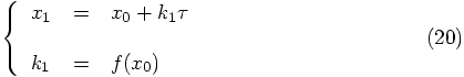
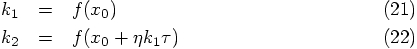
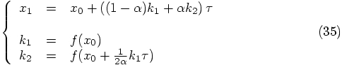
Alice: Now we can move to more interesting venues, when we allow
two force evaluations per step. After a first evaluation of the
right-hand side of the differential equation, we can perform a
preliminary integration in time, after which we can evaluate the
right-hand side again, at a new position:
Alice: Yes. And since that Taylor series for
Bob: The main obstacle here is
Alice: The solution here is that we can develop
Bob: So we have to conclude that our scheme is only second-order
accurate. That makes sense: with one force evaluation, we got a
first-order scheme, and with two force evaluations, we get a
second-order scheme. Presumably with p force evaluations, you get a
scheme that is accurate to order p.
Alice: I would have guessed so too, but this is not so. Your guess
is correct for order 3 and 4, but it turns out that you need 6 force
evaluations to build an algorithm that is accurate to order 5!
Bob: That is surprising!
Alice: It is, until you realize that you get more and more equations that
you have to satisfy. The number of such conditions grows quite a bit
faster than the the number of force calculations. This is not yet obvious
in what we have done, but if will become obvious pretty soon. In general,
there are a lot of complicated combinatorial surprises in Runge-Kutta
derivations.
Bob: Fascinating. But for now, at least, it seems that going to higher
order gives us more freedom, rather than less. Unlike the first-order case,
we now have an extra parameter to play with.
We started with three free parameters,
Alice: Well, let's check. If we define
1.1. Starting at Square One
 scheme that had a misprint in it?
1.2. Keeping it Simple
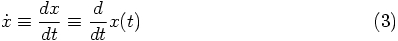
1.3. Notation
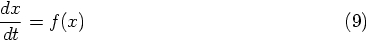
 the position and the
variable
the position and the
variable  the time. The solution of this equation is
given by
the time. The solution of this equation is
given by  . When we solve this equation numerically,
we use a finite time step
. When we solve this equation numerically,
we use a finite time step  . For now, we will analyze
the properties of the first time step. We choose
. For now, we will analyze
the properties of the first time step. We choose  at
the beginning of the first time step, and we denote the positions at
the beginning and end of the first time step by
at
the beginning of the first time step, and we denote the positions at
the beginning and end of the first time step by  and
and
 , respectively:


1.4. A Matter of Interpretation
 a force, but that doesn't seem
right. This equation tells us that the velocity is prescribed, and
equal to
a force, but that doesn't seem
right. This equation tells us that the velocity is prescribed, and
equal to  . A true force would give rise to an
acceleration, not a velocity.
. A true force would give rise to an
acceleration, not a velocity.
 as a velocity.
 , which means that the acceleration is
proportional to the net force acting on the body. You now want to
have a velocity, but you have to specify what it is that is imposing
itself on your particle to produce that velocity.
, which means that the acceleration is
proportional to the net force acting on the body. You now want to
have a velocity, but you have to specify what it is that is imposing
itself on your particle to produce that velocity.
 for the potential energy per unit mass, and
 for the total energy per unit mass, then the velocity
can be expressed as:
for the total energy per unit mass, then the velocity
can be expressed as:

 a force from the beginning.
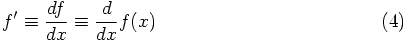
1.5. Taylor Series

1.6. New Force Evaluations
1.7. One Force Evaluation per Step
 :
:


 after we take one step? Let us
see how well we can match Eq. (15) with Eq. (17),
in successive powers of
after we take one step? Let us
see how well we can match Eq. (15) with Eq. (17),
in successive powers of  .
The constant term
.
The constant term  matches
trivially, and our first condition arises
from the term linear in
matches
trivially, and our first condition arises
from the term linear in  :
:

 term in
Eq. (17):
such a match would require
term in
Eq. (17):
such a match would require  ,
which is certainly not true for general force prescriptions.
,
which is certainly not true for general force prescriptions.
1.8. Two Force Evaluations per Step
 . The coefficient
for each term is, as yet, arbitrary, so let us parametrize them as
follows:
. The coefficient
for each term is, as yet, arbitrary, so let us parametrize them as
follows:


 is defined
as a series in
is defined
as a series in  , we must somehow translate the above
expressions, too, a series in
, we must somehow translate the above
expressions, too, a series in  , around
  .
.
 ,
which itself involves an expression that depends on
,
which itself involves an expression that depends on  .
.
 itself in a Taylor series around
  . In general,
for any function of , we can write the Taylor series for a position
. In general,
for any function of , we can write the Taylor series for a position
 near
near  as:
as:


 , we have to insist that


 , we would like to satisfy:

 ? This would require

 , this would require that
  ,
which is not true for general force prescriptions.
,
which is not true for general force prescriptions.
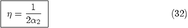
1.9. A One-Parameter Family of Algorithms
 ,
,
 , and
, and  . Since we only have the
two boxed conditions above, we can expect to be left with one degree
of freedom in choosing the coefficients in our algorithm.
. Since we only have the
two boxed conditions above, we can expect to be left with one degree
of freedom in choosing the coefficients in our algorithm.
 , we find:
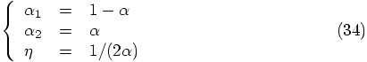

 , leading to:

 , which gives:

 , we effectively average the
evaluations at the beginning and at the end of the trial step, and you
can imagine that this gives you one extra order of accuracy, since you
effectively cancel the types of error you would make if you were using
a force calculation only at one end of the step.
, we effectively average the
evaluations at the beginning and at the end of the trial step, and you
can imagine that this gives you one extra order of accuracy, since you
effectively cancel the types of error you would make if you were using
a force calculation only at one end of the step.
 , we use the evaluation at the
end of a smaller trial step that brings us approximately mid-way
between the beginning and the end of the step. Then, at that point,
we again obtain an estimate for the average of the forces at begin and
end of the time step.
, we use the evaluation at the
end of a smaller trial step that brings us approximately mid-way
between the beginning and the end of the step. Then, at that point,
we again obtain an estimate for the average of the forces at begin and
end of the time step.