2. Recycling Force Evaluations
Alice: So far, we have used up to two force calculations per time step,
independently of what has been done in the previous time step. As we
discussed before, there are situations in which we can recycle a previous
force calculation.
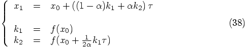
To be specific, taking the result from the previous section,
Eq.(35)
Bob: Not really, no. At least, I don't think so. The first force
calculation for the second step will be evaluated at
Alice: In general, you must be right. But let's not jump to conclusions;
the whole point of our systematic approach is to really make sure that our
hunches are correct, by deriving everything to the point of reaching absolute
certainty.
Bob: what you call systematic others may call tedious, or worse.
Alice: So be it; I just want to be sure. So, for recycling to work in
the strict sense, the position at which
So here is the formal check that your hunch was right!
Bob: This result is not surprising, when we reflect on what
it means: if the equality
Alice: That must be right. The best we can hope for is that
Bob: Lookinging at Eq. (42) as a physicist, rather than a
mathematician, I would start by noting that
Alice: Even though you're a physicist, you should at least show that
this choice brings
Bob: Okay, if you insist. For
Bob: It's clear to me. What else could be better?
Alice: I think I agree, but for future reference, I would like to give a
formal derivation. Soon we will get to much more complicated situations,
where we can't use intuition anymore, and I would like to see exactly how
I can prove that this is the best choice. So bear with me, while I try
to minimize the difference between
Bob: I told you so! And for good measure, let me give you another
physical intuition derivation. At the beginning of the second step,
we can only recycle a previous force if that force was performed at
the end of the previous step. In first approximation, given the force
Alice: Yes, I fully agree that it is helpful to look at the results
from several angles, to get more of a fingertip feeling of what it all
means. Still, I wouldn't have been fully happy without a formal
derivation. But let's move on.
Bob: The question is, can we use our buest guess, or in your case,
best derivation, for recycling?
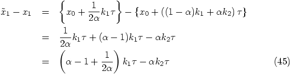
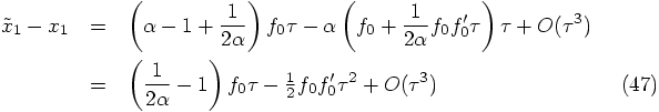
Alice: At first sight, the second-order offset in Eqs. (44)
and (47) may seem problematic, since we are aiming at
developing a second order algorithm, with third-order errors.
However, when we recycle the last force calculation in the next step
we will always use it in multiplication with an extra power of
To show this explicitly, let us extend our notation, using
Bob: Great! So there is a place for recycling, after all. And the
scheme we have found, for
Alice: I didn't either. Normally, it is presented in the text books
as a scheme where you simply have to evaluate the force two times in
every step.
Bob: Most likely, the accuracy will be less per time step. However,
if force evaluation is the most expensive part of the calculation, as
it certainly is for the N-body problem, switching to recycling
allows us to take a step size that is two times smaller, for the same
number of force calculations.
Alice: That probably means that it depends on the particular application
whether recycling is a good idea or not. Making the step size two times
smaller means that the error per step will become eight times smaller, and
the error for a fixed time interval four times smaller, at least
approximately. If the extra error introduced by recycling makes the
calculation error more than four times larger, it is not a good idea.
Bob: At least we have an extra tool in our toolbox. I like gathering
extra algorithms! It would be fun to see under which circumstances we
get a better result.
Alice: But not right now. I prefer to continue first our systematic
investigation with paper and pencil, before we start coding things up
again.
Bob: Fine.
Alice: Let us summarize what we have learned so far.
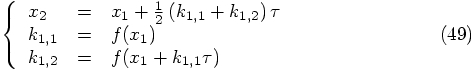
Bob: You would think that we can now add a third force calculation per
step, while recycling the last one. This would mean to new force
calculations and one recycled one per step. And just as we found a
second-order scheme when using one old and one new force, I seems
pretty clear that we can now find a third-order scheme, using one old
and two new forces.
Alice: I agree that that seems likely, but there is no guarantee.
Remember that you can obtain a fourth-order scheme with four forces,
but that a fifth-order scheme requires six forces. These combinatoric
questions cannot be derived by analogy; I'm afraid we just will have to
do the hard work of deriving them.
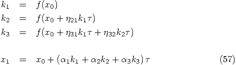
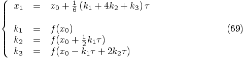
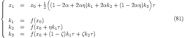
Our first task is to write the form of a general Runge-Kutta scheme
with three force calculations per time step. Once we have this form,
we can insist on the extra condition that the position of the final
force calculation coincides with the position at the beginning of the
next time step, at least to within second order in
The general three-stage Runge-Kutta scheme looks like this:
Bob: This is all nice and fine, but I'd like to see some concrete examples.
Since we have four equations for six unknown variables, we expect to
have a two-parameter freedom of choice. Let's use that freedom, and write
down a few examples, to get a feeling for the type of algorithms we have
at our hands.
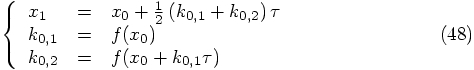
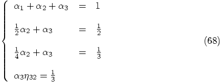
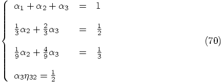
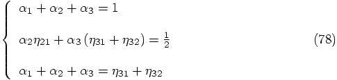
Alice: A natural choice would be to require that the second force
evaluation takes place in the middle of the time step
Let's check that. By substituting our two conditions into the four
boxed equations we found above, we get:
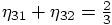
Alice: Another natural choice is to spread the force calculations evenly over
the interval, at times
Bob: Such a scheme obviously cannot be used for our current purposes.
You need the third force calculation at the very end of the step, otherwise
there is nothing to recycle.
Alice: That is true, but you asked for example algorithms, and I expect this
to lead to another well-known scheme, so let us derive it here on the side.
If nothing else, it can function as a check on our calculations.
We require that
Alice: It is time to return to our original objective, to find a third-order
scheme that uses three force calculations per time step, two of which
are computed anew, while the third one is being recycled from its use
in the previous step. With two free parameters, we seem to have a
good chance to find such a scheme.
As in Eqs. (45) and (47), we have to calculate the
difference between the position
Alice: Not so fast. Don't count your chickens before they are hatched!
Bob: I haven't heard that expression in a long time. Well, hatching
shouldn't be too difficult.
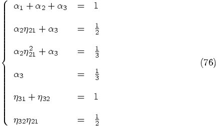
Alice: Gathering all six equations, we get:
Bob: So far, so good.
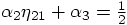
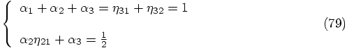
Alice: Or so it seems. Look, when we substitute the
fourth relation into the second and third one, we obtain:
The last line implies that either
Bob: I guess hatching was unsuccessful. That's a disappointment!
Alice: We have to conclude, somewhat surprisingly, that there just is no
third-order recycling scheme. Whether we use two new force
calculations per time step, or whether we recycle an additional force
calculation from the previous time step, in both cases we wind up with
a second-order algorithm.
Bob: That's a pity.
Alice: However, not all is lost: our scheme is still second-order, and has
more freedom than our non-recycling scheme. Specifically, let us
gather the set of conditions necessary to guarantee at least
second-order behavior for our recycling method. These are, from
Eqs. ((64), ((65), and ((74):
Bob: I'm not sure whether we've gained anything, by getting extra free
parameters. I had hoped for a third-order scheme.
Alice: We haven't gained anything, but neither have we lost anything.
Later, when we will apply these various algorithms, we can check to see
whether any of the new parameters allow choices that give us more
accurate results.
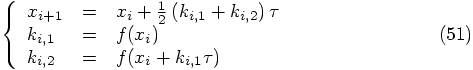
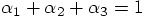
We can compare Eq. (81) with the non-recycling schemes, where we
also perform two force calculations per step, and for which we
obtained a second-order scheme as well. We found there, as Eq.(35):
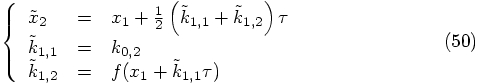
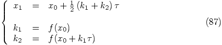
Alice: It is also instructive to compare this scheme with the
second-order scheme we found based on one new force calculation and
one recycled force calculation:
Alice: Let us sum up.
We conclude that we have found three different ways of constructing a
second-order Runge-Kutta method:
2.1. One Force Evaluation per Step
 of
the first step, and to recycle its use, to let it function as the
of
the first step, and to recycle its use, to let it function as the
 contribution to the second step?
 ,
the end point of the first step. However, the last force calculation
for the first step was not evaluated at that exact point. Rather it
was evaluated at the point that was reached by using only the information
given by
,
the end point of the first step. However, the last force calculation
for the first step was not evaluated at that exact point. Rather it
was evaluated at the point that was reached by using only the information
given by  .
.
 is calculated
during the first step should coincide with the position at which
is calculated
during the first step should coincide with the position at which
 needs to be calculated during the second step.
Let us define that first position as
needs to be calculated during the second step.
Let us define that first position as  , which
means that
, which
means that  , which implies
 :
:


 , this
expression should hold for arbitrary values of
, this
expression should hold for arbitrary values of  and
and
 . If we first look at the dependence on
  ,
we find
,
we find  and therefore
  .
But this then implies that
.
But this then implies that  , which is not true in general.
 would hold exactly,
there would be no reason to compute the last force evaluation. For this
reason, there should not be any Runge-Kutta scheme that allows strict
recycling of a force evaluation, come to think of it.
would hold exactly,
there would be no reason to compute the last force evaluation. For this
reason, there should not be any Runge-Kutta scheme that allows strict
recycling of a force evaluation, come to think of it.
2.2. What is Good Enough?
 is reasonably accurate as a predicted value,
good enough, so to speak. Now the question is whether we can find a
precise meaning for `good enough.' What does it mean for
is reasonably accurate as a predicted value,
good enough, so to speak. Now the question is whether we can find a
precise meaning for `good enough.' What does it mean for
 not to differ too much from the corrected value
 ?
?
 ,
at least in the limit of a small time step. This suggests that the
best we can do is to let the right hand side disappear, through the
choice
,
at least in the limit of a small time step. This suggests that the
best we can do is to let the right hand side disappear, through the
choice  . In that case, the left-hand side
will still not be exactly zero, but it will be small.
. In that case, the left-hand side
will still not be exactly zero, but it will be small.
 and
and  close
together. Handwaving alone is certainly not good enough!
close
together. Handwaving alone is certainly not good enough!
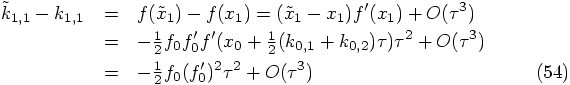
 we can
determine the difference between the two force evaluations as:
we can
determine the difference between the two force evaluations as:

 and
and
 directly, starting from the most general form:
 and use the expansion

 is the best approximation, and
the remaining term is second order in
is the best approximation, and
the remaining term is second order in  .
.
 at
at  , we can write
 . Comparing this with
Eq. (38), we see immediately that
. Comparing this with
Eq. (38), we see immediately that  , hence
  .
.
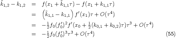
2.3. Approximate Recycling
 .
This means that the slight offset will cause only third order errors,
on the same level of the truncation errors we are making anyway.
.
This means that the slight offset will cause only third order errors,
on the same level of the truncation errors we are making anyway.
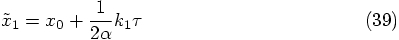
 to denote
  for the step starting at
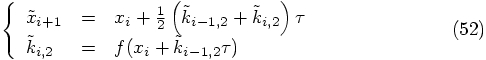
  , and let us use tildes
to indicate the approximate solution that we obtain when we recycle
the previous force evaluation. Here are the expressions for the first
step:
, and let us use tildes
to indicate the approximate solution that we obtain when we recycle
the previous force evaluation. Here are the expressions for the first
step:
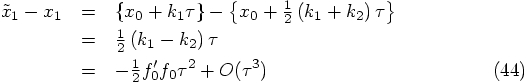
 and
and
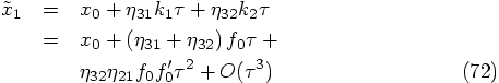
 is of third order in
  , as we can
illustrate by evaluating down the differences in position at the end of
the second step:
, as we can
illustrate by evaluating down the differences in position at the end of
the second step:


 . Since our basic algorithm is only
second-order accurate in
. Since our basic algorithm is only
second-order accurate in  per step, the only effect
is to change the magnitude of the leading error term, without
affecting the second-order nature of the algorithm.
per step, the only effect
is to change the magnitude of the leading error term, without
affecting the second-order nature of the algorithm.
2.4. Summary
 is just one of the
classic second-order Runge-Kutta schemes, the one we already wrote
down in Eq. (36). I had no idea that that algorithm
could be used in a recycling fashion.
is just one of the
classic second-order Runge-Kutta schemes, the one we already wrote
down in Eq. (36). I had no idea that that algorithm
could be used in a recycling fashion.
 , also given above as
Eq. (36).
, also given above as
Eq. (36).
2.5. Two Force Evaluations per Step
 .
.


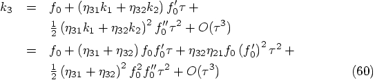


 the relation

 we find

 involving the second derivative of
the force, we find
involving the second derivative of
the force, we find

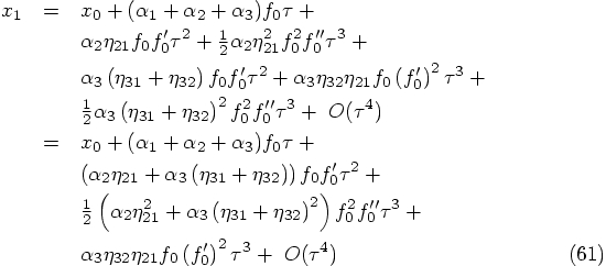
 involving the square of the
first derivative of the force, we find
involving the square of the
first derivative of the force, we find

2.6. Two Examples
 , while the third force evaluation
takes place at the end of the step
, while the third force evaluation
takes place at the end of the step 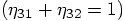 .
With these two extra conditions, barring unforeseen complications, we
can expect to find a unique solution.
.
With these two extra conditions, barring unforeseen complications, we
can expect to find a unique solution.
 and
and  ,
after which the first equation yields
,
after which the first equation yields  .
The last equation then gives
.
The last equation then gives  which implies
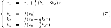
 . We thus arrive at the following
third-order scheme:
. We thus arrive at the following
third-order scheme:
 ,
,  , and
, and
 , before starting the calculations for the new
step at time
, before starting the calculations for the new
step at time  .
.
 and
and
 . Plugging this into the
four conditions we have found before leads to:
. Plugging this into the
four conditions we have found before leads to:
 and
and
 , and whith the first equation we find
 . The last equation yields
 which then determines
 . We thus arrive at:
2.7. Recycle Conditions
 at which the last force
calculation of the previous step took place and the actual position
at which the last force
calculation of the previous step took place and the actual position
 at the end of that step. In Eq. (47) we only needed to
let the term linear in
at the end of that step. In Eq. (47) we only needed to
let the term linear in  vanish, in order to obtain a consistent
second-order scheme. In the present case, for a third-order scheme,
we need to let both the linear and quadratic terms in
vanish, in order to obtain a consistent
second-order scheme. In the present case, for a third-order scheme,
we need to let both the linear and quadratic terms in  vanish.
Using Eq. (59), we have:
vanish.
Using Eq. (59), we have:
 :
:

 and
and  to match in the last
two equations gives us two extra conditions:
to match in the last
two equations gives us two extra conditions:


 .
.
 and
another one in simplified form as
and
another one in simplified form as
 into the last two boxed equations.
 or
or
 . Either case would imply
 , in contradiction with
the requirement that
, in contradiction with
the requirement that  .
.
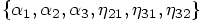
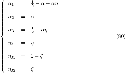
2.8. Remaining Freedom
 ,
,  , and
, and
 , we get the following parametrized solutions:
2.9. Summary

 in the calculation of the
new position. This means:
in the calculation of the
new position. This means:


 ,
the expression for the second force becomes:
,
the expression for the second force becomes:

 ,
Eq. (81) becomes Eq. (82). It all hangs together! The
third force calculation in Eq. (81) effectively drops out, for
this choice of parameters.
,
Eq. (81) becomes Eq. (82). It all hangs together! The
third force calculation in Eq. (81) effectively drops out, for
this choice of parameters.
 .
.
Bob: Well done! Now it's time to leave this first-order differential
equation behind us. I think we've learned enough, and I would prefer to
go to the more realistic case of a second-order differential equation.