4. Partitioned Runge-Kutta Algorithms
Bob: You promised a better approach to solving second-order differential equations, using Runge-Kutta schemes. What did you call such an algorithm again?
Alice: It is called a partitioned Runge-Kutta algorithm. The idea is to
combine the force calculations in different ways for the position and for
the velocity. The word `partitioned' here means that separate the treatment
of  from the treatment of
  . We already saw
an example at the end of our previous discussion, where we had found a
scheme that was almost, but not quite, a leapfrog scheme. If we would have
tinkered with that scheme, we could have turned it into a leapfrog,
but it would then no longer be a vector generalization of a
Runge-Kutta scheme.
. We already saw
an example at the end of our previous discussion, where we had found a
scheme that was almost, but not quite, a leapfrog scheme. If we would have
tinkered with that scheme, we could have turned it into a leapfrog,
but it would then no longer be a vector generalization of a
Runge-Kutta scheme.
Bob: So you're saying that we have a lot more freedom, when we allow separate ways to update position and velocity, after first calculation a number of force evaluations.
Alice: Exactly. And we have already done this, for our fourth-order integrator, the one we plucked from Abramowitz and Stegun.
Bob: Does this mean that we can write our good old leapfrog as a partitioned Runge-Kutta scheme? That would be interesting! I have always thought about Runge-Kutta methods and the leapfrog scheme as two completely different animals, pardon the pun. Do you think that the leapfrog can be view as a type of Runge-Kutta algorithm?
Alice: I'm not sure. One reason to do this systematic landscape exploration is to find the answers to that type of question! And I'm sure we'll find out soon. By exploring all possible schemes with up to two new force calculations per step, we're bound to encounter the leapfrog, if indeed it is a citizen of the Runge-Kutta world.
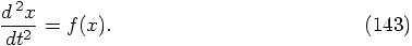
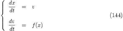
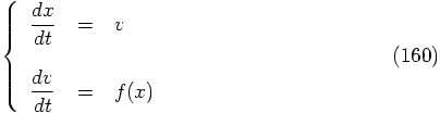
So let us return to our special second-order differential equation

Bob: I guess we will forget about force recycling, at least for now.
Alice: Yes. To keep things simple, let us look at a single integration
step. But we have another choice to make.
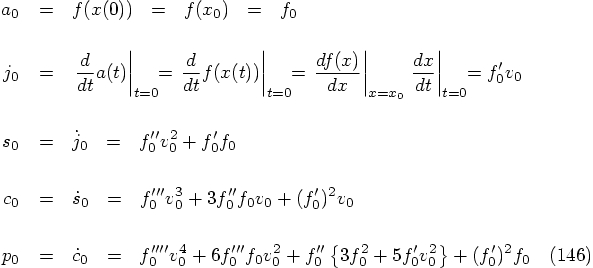
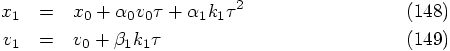
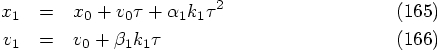
In the case of a first-order differential equation, at the start of
our integration we can only evaluate the right-hand side at time zero,
at the beginning of the integration time step. If we simply follow
that example, we start with:
Looking now at the velocity, we have
Bob: And I presume that there is no point in using a higher-order algorithm
for the position than for the velocity, since the overall order of the
integration scheme must be the lowest order of that of the components.
Hmmm. Is that so?
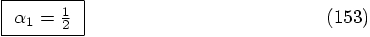
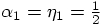
Alice: Yes, that is correct. For the very first step, it is possible in
this case to find a new position that is second-order accurate. But
as soon as we take the second step, we use the velocity that we arrived
at in the first step, which is only first-order accurate. The same is
true for each subsequent step: we always use the velocity value from
the previous step.
Bob: But each time we multiply the velocity with
Alice: Yes, that is formally correct. However, \dots
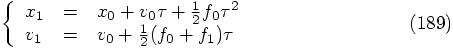
We have to conclude that our approach only leads to a first-order correct
algorithm, which is of course the forward Euler algorithm:
{\bf 4.1.1.2. A Delayed Force Evaluation}
Given the special form of our second-order differential equation, it
is not necessary to start with a force evaluation at time zero. The
first equation in the set
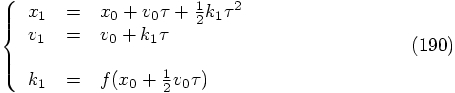
Let us exploit this extra freedom, for our special differential equation,
by repeating our previous analysis for a delayed force evaluation.
Our first force evaluation can now take place at time
let us first consider the
Considering the
Could it be that we are in luck, and that this fixed solution can give
us expressions for
%\subsubsubsection{Verlet-St\"ormer-Delambre Scheme}
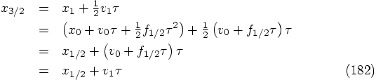
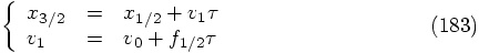
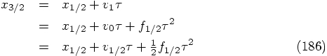
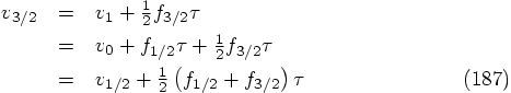
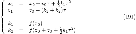
{\bf 4.1.1.3. Verlet-St\"ormer-Delambre Scheme}
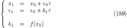
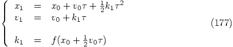
Using one evaluation of the right-hand side of the differential equation,
we have thus arrived at the following second-order integration scheme:
In fact, this scheme is nothing else than the good old leapfrog
algorithm, also known as the Verlet-St\"ormer-Delambre scheme, as we
will show now.
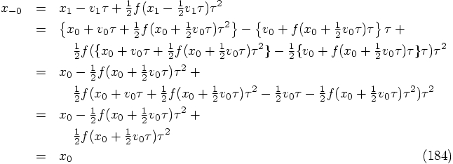
Define
%\subsubsubsection{An Historical Note}
{\bf 4.1.1.4. An Historical Note}
Almost everywhere in the literature, Runge-Kutta methods are assumed
to start with
In his section 2, p. 7, near the bottom, he remarks that, to be
consistent, we should allow the freedom to write a general expression
of the type we have done above in Eq. (164). He then adds that
he decided against considering this extra freedom, for two reasons,
both pragmatic, the first related to speed of execution of the
algorithms, the second related to speed of derivation of the
expressions fot the algorithms. Here are his arguments.
First of all, we often know already the force evaluation at the
beginning of the step, from the last stage of the calculation of the
previous step (at least approximately; and using even earlier force
calculations, we can further improve the accuracy, without having to
perform new force evaluations). Secondly, he adds, starting from such
a general expression has led him to such unwieldy expressions that he
was more or less forced to put
Of course, current availability of algebraic manipulation programs
have now invalidated his second argument. Curiously, all text books
seem to propagate the simplifying assumption
%\subsubsubsection{General Form}
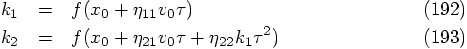
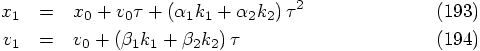
{\bf 4.1.2.1. General Form}
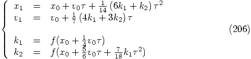
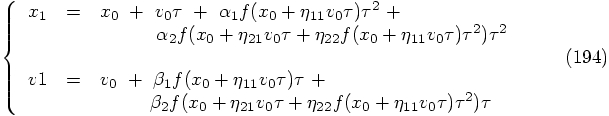
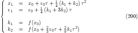
If we allow two evaluations of the right-hand side of the differential
equation, we can work with the following general expression that is
dimensionally correct
4.1. One Force Evaluation per Step

 , as
, as


 , so as far
as the expression for the position is concerned, we can make our scheme
second-order accurate.
, so as far
as the expression for the position is concerned, we can make our scheme
second-order accurate.


 :
:

 would require that

 and
and  .
Even though we can construct a second-order algorithm for the position,
we can only find a first-order algorithm for the velocity.
.
Even though we can construct a second-order algorithm for the position,
we can only find a first-order algorithm for the velocity.
 .
So even though the velocity is first-order, the product of the velocity
with
.
So even though the velocity is first-order, the product of the velocity
with  must be second-order correct, leading to an error
term that is third-order in
must be second-order correct, leading to an error
term that is third-order in  .
.


 at
time zero, before we can perform a subsequent force evaluation at time
at
time zero, before we can perform a subsequent force evaluation at time  .
.
4.2. xxx
 where
where  is a free parameter. Using the linear extrapolation of
the position, as sketched above, we obtain:
is a free parameter. Using the linear extrapolation of
the position, as sketched above, we obtain:

 to first order in
  , we obtain:


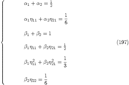
 terms, which leads to the
requirement:
terms, which leads to the
requirement:


 :
:

 term, we have:


 terms, we have:


 in both position and velocity.
 and
and  that are also third-order correct in
  ?
Let us start with the position equation. This would require:
?
Let us start with the position equation. This would require:

 , the
coefficient on the right-hand side is
, the
coefficient on the right-hand side is  while the one on the
left-hand side is
while the one on the
left-hand side is  . We have no freedom left, so this equation has
no solutions for a general function
. We have no freedom left, so this equation has
no solutions for a general function  and a general initial velocity
  .
.
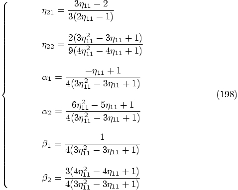
 and
and  are determined.


 ,
which are obtained from
,
which are obtained from  by taking a time step with
size
by taking a time step with
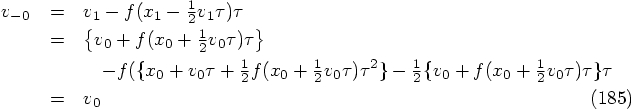
size  . Our task is to show that
  actually
coincide with
actually
coincide with  , not only to second order, as would
be guaranteed in any second order scheme, but in fact to all orders in
, not only to second order, as would
be guaranteed in any second order scheme, but in fact to all orders in
 .
.

 : letting the first evaluation of the
right-hand side of the differential equation take place at the very
beginning of the step. This is necessary in the general case, but not
for the special case of a second-order differential equation where
there is no velocity dependence in the force term. The only place we
have found so far in the literature, which mentions the possibility of
starting with the force evaluation already at a later time is a
paragraph in
: letting the first evaluation of the
right-hand side of the differential equation take place at the very
beginning of the step. This is necessary in the general case, but not
for the special case of a second-order differential equation where
there is no velocity dependence in the force term. The only place we
have found so far in the literature, which mentions the possibility of
starting with the force evaluation already at a later time is a
paragraph in  (1925),
the original paper introducing what is
now known as the
(1925),
the original paper introducing what is
now known as the  algorithms.
 in his equivalent to our
Eq. (164).
in his equivalent to our
Eq. (164).
 without
questioning what the basis for this assumption may have been.
without
questioning what the basis for this assumption may have been.
4.3. Two Force Evaluations per Step
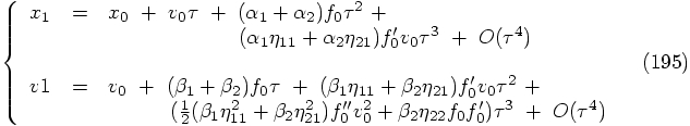
 values, these equations expand into
 , we get:

 , as follows:
 , we get:

 (1925) gives this as his simplest
algorithm:
(1925) gives this as his simplest
algorithm:
 (1925).
However, Henrici's expressions contain a typo: he lists the last
coefficient as
(1925).
However, Henrici's expressions contain a typo: he lists the last
coefficient as  .
.
 does list the term correctly,
as
does list the term correctly,
as  .
.
 , we find that
some of the coefficients diverge:
, we find that
some of the coefficients diverge: 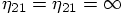 .
With two force evaluations, it seems not to be possible to let the
first one start right in the middle.
.
With two force evaluations, it seems not to be possible to let the
first one start right in the middle.
 .
Here the first force evaluation takes place after one third of the
duration of the time step. In this case we get:
.
Here the first force evaluation takes place after one third of the
duration of the time step. In this case we get:

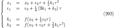
 , for which the first
force evaluation takes place after two third of the duration of the
time step. In this case we get:
, for which the first
force evaluation takes place after two third of the duration of the
time step. In this case we get:

 ,
but in that case we get the much more complicated looking set:
,
but in that case we get the much more complicated looking set: