1. A Surprising Algorithm
Alice: We have been quite busy with our project to lay the foundations
for a N-body simulation environment.
Bob: I'd say! It seems like ages since we did some actual N-body
calculations. We started with the two-body problem . . .
Alice: . . . and then you got carried away, adding one integrator after
another, before we finally moved on to the general N-body problem . . .
Bob: . . . at which point you told us to stop moving, and to lay
foundations instead! I feel like we turned into computer scientists
instead of astrophysicists.
Alice: I'm afraid we had no choice. The alternative would have been
to come up with stopgap solutions at every turn in the road. Now at least
we have a reliable and flexible data format and corresponding I/O routines,
and we have a library structure that allows us to organize our codes. And
even before we built that, we introduced extendable command line options
that maked our codes self-describing through a detailed help facility.
Bob: I must admit, all those features do make life easier. I remember
getting rather tired, editing a file each time I wanted to perform a
different run, before we had command line options. That seems like a
long time ago! Okay, where were we?
Alice: In volume ???acsio??? we had collected the various integrators in a
single file nbody_cst1.rb, while we were getting the ACS data format
straightened out. Let us start from the same file, in this new directory,
corresponding to the current volume.
Bob: And let us start by calling it nbody_cst1a.rb, so that we
can experiment with a few versions 1a, 1b, etc, until we are happy with a
more stable version, which we can then call nbody_cst1.rb again,
in this directory. At that point, we can export that version once more
to our "bin/kali" directory.
Alice: Do you remember how to run nbody_cst1a.rb?
Bob: Don't have to! Remember, we had a ---help option, which
should give not only a detailed description of what the codes does, but in
addition it should give a simple example invocation.
Alice: Ah, yes, that's one of the nifty features we added. We've sure done
a lot! Let's try:
Alice: That all seems quite reasonable. And we do have quite a number of
different algorithms implemented, by now. Shall we move on, from constant
time steps to adaptive time steps, and after that, to individual time steps?
Bob: Yes, we should do that soon. However, before moving on, let me show
you a paper that I stumbled upon, by Sia. A. Chin and C. R. Chen.
I found it on astro-ph, under
astro-ph/0304223.
This paper presents an algorithm that is totally different from what
I've seen so far.
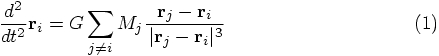
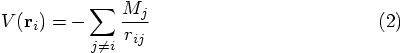
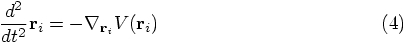
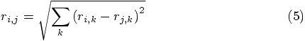
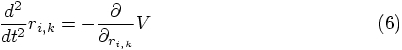
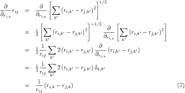
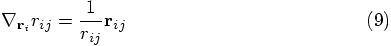
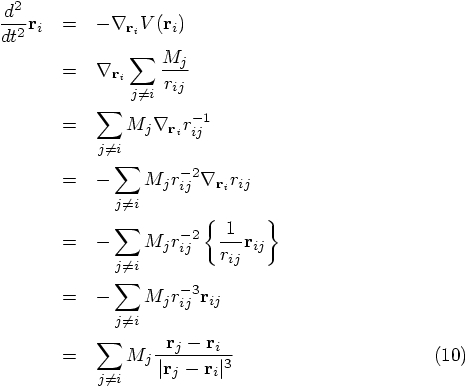
Let me remind you how this equation can be derived, starting with the
gravitational potential
1.1. Picking up the Pieces
 |gravity> kali nbody_cst1a.rb ---help

     This program evolves an N-body code with a fourth-order Hermite Scheme,
     or various other schemes such as forward Euler, leapfrog, or Runge-Kutta,
     using constant time steps, shared by all particles, where the size of
     of the time step is prescribed beforehand.  The program includes the
     option to provide softening for the potential.  This is essential for
     a constant time step code; the alternative, instead of softening, would
     be to use a variable time step algorithm.

     (c) 2005, Piet Hut and Jun Makino; see ACS at www.artcompsi.org

     example:
     kali mkplummer.rb -n 4 -s 1 | kali nbody_cst1a.rb -t 1 > /dev/null
Well, let's follow the advice:
 |gravity> kali mkplummer.rb -n 4 -s 1 | kali nbody_cst1a.rb -t 1 > /dev/null
 ==> Plummer's Model Builder <==
 Number of particles            : N = 4
 pseudorandom number seed given : 1
 Screen Output Verbosity Level  : verbosity = 1
 ACS Output Verbosity Level     : acs_verbosity = 1
 Floating point precision       : precision = 16
 Incremental indentation                : add_indent = 2
              actual seed used  : 1
 ==> Constant Time Step Code <==
 Integration method             : method = hermite
 Softening length               : eps = 0.0
 Time step size                 : dt = 0.001
 Interval between diagnostics output: dt_dia = 1.0
 Time interval between snapshot output: dt_out = 1.0
 Duration of the integration    : t = 1.0
 Screen Output Verbosity Level  : verbosity = 1
 ACS Output Verbosity Level     : acs_verbosity = 1
 Floating point precision       : precision = 16
 Incremental indentation                : add_indent = 2
 at time t = 0, after 0 steps :
   E_kin = 0.25 , E_pot =  -0.5 , E_tot = -0.25
              E_tot - E_init = 0
   (E_tot - E_init) / E_init = -0
 at time t = 1, after 1000 steps :
   E_kin = 0.248 , E_pot =  -0.613 , E_tot = -0.365
              E_tot - E_init = -0.115
   (E_tot - E_init) / E_init = 0.461
1.2. The Chin and Chen paper
1.3. xxx

 , and
similarly for the other vectors. The last equations then become:
, and
similarly for the other vectors. The last equations then become:
 and therefore

1.4. xxx
 , which implies
