1. Leapfrog
Alice: Hi, Bob! Any luck in getting a second order integrator to work?
Bob: No problem, it was easy! Actually, I got two different ones to
work, and a fourth order integrator as well.
Alice: Wow, that was more than I expected!
Bob: Let's start with the second order leapfrog integrator.
Alice: Wait, I know what a leapfrog is, but we'd better make some
notes about how to present the idea to your students. How can we do
that quickly?
Bob: Let me give it a try. The name leapfrog comes from one
of the ways to write this algorithm, where positions and velocities
`leap over' each other. Positions are defined at times
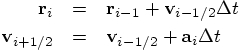
A second way to write the leapfrog looks quite different at first sight.
Defining all quantities only at integer times, we can write:
Alice: A great summary! I can see that you have taught numerical
integration classes before. At this point an attentive student might
be surprised by the difference between the two descriptions, which you
claim to describe the same algorithm. They may doubt that they really
address the same scheme.
Bob: How would you convince them?
Alice: An interesting way to see the equivalence of the two descriptions
is to note the fact that the first two equations are explicitly
time-reversible, while it is not at all obvious whether the last two
equations are time-reversible. For the two systems to be equivalent,
they'd better share this property. Let us inspect.
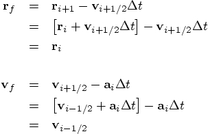
Starting with the first set of equations,
even though it may be obvious, let us write out the time reversibility.
We will take one step forward, taking a time step
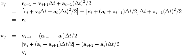
Now the real fun comes in, when we inspect the equal-time version, the
second set of equations you presented:
Bob: A good exercise to give them. I'll add that to my notes.
Alice: Now show me your leapfrog, I'm curious.
Bob: I wrote two new drivers, each with its own extended Body class.
Let me show you the simplest one first. Here is the leapfrog driver
integrator_driver1.rb:
Same as before, except that now you can choose your integrator.
The method evolve, at the end, now has an extra parameter,
namely the integrator.
Alice: And you can supply that parameter as a string, either
"forward" for our old forward Euler method, or "leapfrog" for your
new leapfrog integrator. That is very nice, that you can treat
that choice on the same level as the other choices you have to make
when integrating, such as time step size, and so on.
Bob: And it makes it really easy to change integration method:
one moment you calculate with one method, the next moment with another.
You don't even have to type in the name of the method: I have written
it so that you can switch from leapfrog back to forward Euler with two
key strokes: you uncomment the line
and comment out the line
Alice: It is easy to switch lines in the driver, but I'm really curious
to see how you let Ruby actually make that switch in executing the code
differently, replacing one integrator by another!
1.1. The Basic Equations
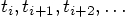 , spaced at constant intervals
 , while the velocities are defined at times halfway in
between, indicated by
, while the velocities are defined at times halfway in
between, indicated by 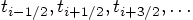 ,
where
,
where  .
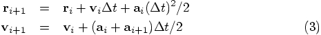
The leapfrog integration scheme then reads:
.
The leapfrog integration scheme then reads:
 are defined only on integer
times, just like the positions, while the velocities are defined only on
half-integer times. This makes sense, given that
are defined only on integer
times, just like the positions, while the velocities are defined only on
half-integer times. This makes sense, given that
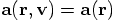 :
the acceleration on one particle depends only on its position with respect
to all other particles, and not on its or their velocities. Only at
the beginning of the integration do we have to set up the velocity at
its first half-integer time step. Starting with initial conditions
:
the acceleration on one particle depends only on its position with respect
to all other particles, and not on its or their velocities. Only at
the beginning of the integration do we have to set up the velocity at
its first half-integer time step. Starting with initial conditions
 and
and  ,
we take the first term in the Taylor series expansion to compute the
first leap value for
,
we take the first term in the Taylor series expansion to compute the
first leap value for  :
:

 , using the first leap value for
 .
Next we compute the acceleration
.
Next we compute the acceleration  , which enables us
to compute the second leap value,
, which enables us
to compute the second leap value,  , using the
second equation above, and then we just march on.
, using the
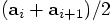
second equation above, and then we just march on.
 is
given by the time step multiplied by
is
given by the time step multiplied by
 , effectively
equal to
, effectively
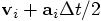
equal to  . Similarly, the increment in
 is given by the time step multiplied by
 , effectively equal to the
intermediate
value
, effectively equal to the
intermediate
value  . In conclusion, although both
positions and velocities are defined at integer times, their
increments are governed by quantities approximately defined at
half-integer values of time.
. In conclusion, although both
positions and velocities are defined at integer times, their
increments are governed by quantities approximately defined at
half-integer values of time.
1.2. Time reversibility
 ,
to evolve
,
to evolve 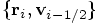 to
to
 , and then we
will take one step backward, using the same scheme, taking a time
step
, and then we
will take one step backward, using the same scheme, taking a time
step  . Clearly, the time will return to the
same value since
. Clearly, the time will return to the
same value since  , but we have to
inspect where the final positions and
velocities
, but we have to
inspect where the final positions and
velocities  are
indeed equal to their initial values
are
indeed equal to their initial values
 . Here is the
calculation, resulting from applying the first set of equations twice:
. Here is the
calculation, resulting from applying the first set of equations twice:
1.3. A New Driver
##method = "forward" # integration method
method = "leapfrog" # integration method