5. A Complete Derivation
Bob: You have a very determined look in your eyes.
Alice: Yes, I feel determined. I want to know for sure that the
integrator listed in Abramowitz and Stegun is fourth-order, and I
want to prove it.
In the form given in their book, they are dealing with a force that
has the most general form: it depends on position, velocity, and time.
In our notation, their differential equation would read
Alice: That is true, but I would like to prove their original formula.
Bob: I don't think that is necessary. We don't have any magnetic force,
or anything else that shows forces that depend on velocity.
Alice: Yes, but now that we've spotted what seems like a mistake, I don't
want to be too facile. Okay, let's make a compromise. I'll drop the
velocity dependence; hopefully our derivation, if successful, should
point the way to how you could include that extra dependence. But I would
like to keep the time dependence, just to see for myself how that mixes
with the space dependence.
And if you want a motivation: imagine that our star cluster is suspended
within the background tidal field of the galaxy. Such a field can be treated
as a slowly varying, time-dependent perturbation, exactly of this form:
Alice: If we really wanted to be formally correct, we could track
the four-dimensional variations in space and time, taking into account
the three-dimensional spatial gradient of the interaction terms.
Bob: But from the way you just said that, I figure that that would be
too much, even for you. I'm glad to hear that even you have your limits
in wanting to check things analytically!
Alice: I sure have. And also, I don't think such a formal treatment
would be necessary. If we can prove things in one dimension, I'm convinced
that we could rewrite our proof to three dimensions without too many problems,
albeit with a lot more manipulations.
Bob: You won't hear me arguing against simplification!
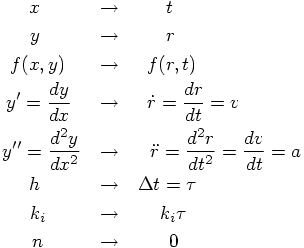
But I propose that we use a somewhat more intuitive notation than what
Abramowitz and Stegun gave us. To use x to indicate time and y to
indicate position is confusing, to say the least. Let us look at the
text again:
How about the following translation, where the position r, velocity v,
and a are all scalar quantities, since we are considering an effectively
one-dimensional problem:
Alice: Yes, I find that notation much more congenial, and I'm glad to see
the explicitly space and time dependence now in the definitions of the three
k variables.
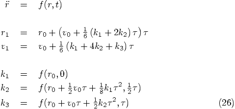
Let us work out what these k variables actually look like, when we
substitute the orbit dependence in the right hand side. What we see
there is an interesting interplay between a physical interaction term
f that has as an argument the mathematical orbit
Since you have introduced
What I propose to do now is to expand
Bob: How do you do a two-dimensional Taylor series expansion?
Alice: Whenever you have mixed derivatives, such as
Bob: That's going to be quite messy.
Alice: Well, yes, but we have no choice. Let me start with
the substitution indicated in Eq. (27), where we may as well
replace
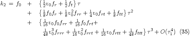
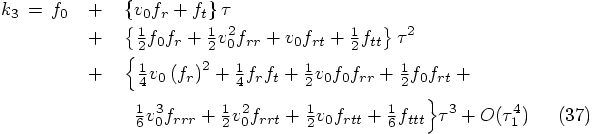
Alice: Yes, that must be right. Okay, ready for a next round of
substitution? Eq. (33) then becomes:
Starting with the position, we find:
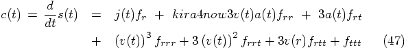
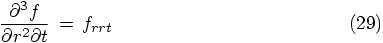
Bob: And the last term in curly brackets, in the first line of the
last equation must be the jerk. I begin to see some structure in these
expressions.
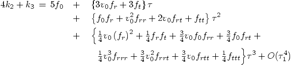
Alice: Yes. But let me get the velocity as well, and then we can take
stock of the whole situation. Let's see. To solve
for
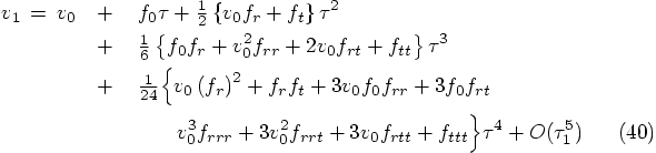
Alice: And an expression that makes sense: we see that indeed the
velocity, Eq. (40),
is the time derivative of the position, Eq. (38), up to the order given
there. So everything is consistent.
Bob: But this is really astonishing. Why would this last expression
be also fourth-order accurate? Even if the fourth-order term had been
totally wrong, the velocity in Eq. (40) would still have been the
time derivative of Eq. (38), up to the accuracy to which that
expression holds. We had no right to expect more!
Alice: It is quite remarkable. But I presume that whoever derived this
equation know what he or she was doing, in choosing the right coefficients!
Well, most likely a he, I'm afraid. I think this equation goes back
to a time in which there were even fewer women in mathematics than
there are now.
Bob: Now that you mention it, I do wonder who derived this marvel. It
still surprises me, that you really can get fourth-order accurate, while
using only three function evaluations.
Alice: Yes, that is neat. It must have something to do with the fact
that we are dealing with a second-order equation. Even though the force
term for the acceleration, as the derivative of the velocity, can be
arbitrarily complex, the derivative of the position couldn't be simpler:
it is always just the velocity.
Bob: I bet you're right. After all, Abramowitz and Stegun list this
algorithm specifically under the heading of second-order differential
equations. They must have had a reason.
Alice: I'd like to trace the history, now that we've come this far.
But first, let's fiish our derivation.
Bob: I thought we had just done that? We've shown that both position
and velocity are fourth-order accurate.
Alice: Well, yes, but by now I've grown rather suspicious. We have
already seen instances where a derivation looked perfect on paper, but
then it turned out to be only formally valid, and not in practice.
Bob: Hard to argue with that!
Alice: What we have done now is to compute the predicted positions and
velocities after one time step, and we have checked that if we vary the
length of the time step, we indeed find that the velocity changes like the
time derivative of the position. The question is: are they really solutions
of the equations of motion that we started out with, up to the fourth order
in the time step size?
Let us go back to the equations of motion, in the form we gave them
just after we translated the expressions from Abramowitz and Stegun:
Alice: And now we have derived them in a fully space-time dependent
way.
Bob: Congratulations! I'm certainly happy with this result. But I must
admit, I do wonder whether this conclusion would satisfy a
mathematician working in numerical analysis.
Alice: Probably not. Actually, I hope not. I'm glad some people are more
careful than we are, to make sure that our algorithms really do what
we hope they do. At the same time, I'm sure enough now that we have a
reasonable understanding of what is going on, and I'm ready to move on.
Bob: I certainly wouldn't ask my students to delve deeper into this matter
than we have been doing so far. At some point they will have to get results
from their simulations.
Alice: At the same time, unless they have a fair amount of understanding
of the algorithms that they rely on, it will be easy for them to use those
algorithms in the wrong way, or in circumstances where their use is
not appropriate. But I agree, too much of a good thing may simply be
too much. Still, if a student would come to be with a burning curiosity
to find out more about what is really going on with these
higher-order integration methods, I would encourage that him or her to
get deeper into the matter, through books or papers in numerical analysis.
Bob: I don't think that is too likely to happen, but if such students
appear on my doorsteps, I'm happy to send them to you!
Alice: And I would be happy too, since I might well learn from them.
I've the feeling that we've only scratched the surface so far.
5.1. The One-Dimensional Case


5.2. A Change in Notation

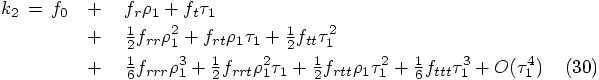
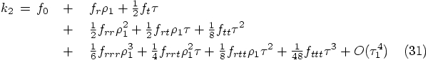
5.3. The Auxiliary k Variables
 .
.
 as the increment in time,
starting from time zero, let me introduce the variable
as the increment in time,
starting from time zero, let me introduce the variable  to indicate the increment in space, the increment in position at the time
that we evaluate
to indicate the increment in space, the increment in position at the time
that we evaluate 


 .
Let me also abbreviate
.
Let me also abbreviate 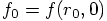 .
.
 in a double Taylor
series, simultaneously in space and in time. This will hopefully repair
the oversight we made before, when we only considered a time expansion.
in a double Taylor
series, simultaneously in space and in time. This will hopefully repair
the oversight we made before, when we only considered a time expansion.
 , we can also write this as

 , for which we get:
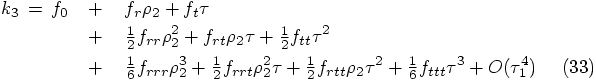
 variables in the
  equations,
and to keep terms up to the third order in
equations,
and to keep terms up to the third order in  .
.
5.4. The Next Position
 by its value
  :
:

 that we just derived, up till third
order in
that we just derived, up till third
order in  , as;
, as;

 that they appear, in the form of partial derivatives
of the interaction term.
that they appear, in the form of partial derivatives
of the interaction term.
 and
and  in the expressions for
 and
and  .
.

5.5. The Next Velocity
 in Eq. (26), we need to use the following
combination of
in Eq. (26), we need to use the following
combination of  values:
 in Eq. (26),
we get:
in Eq. (26),
we get:
5.6. Everything Falls into Place


 , to find the jerk:


 , we find the snap:

 :
:

 ,
we can derive the crackle:
,
we can derive the crackle: