8. A Two-Step Method
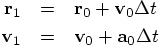
Bob: So far we have used only one-step methods: in each case we start
with the position and velocity at one point in time, in order to calculate
the position and velocity at the next time step. The higher-order
schemes jump around a bit, to in-between times in case of the traditional
Runge-Kutta algorithms, or slightly before or beyond the one-step interval
in case of Yoshida's algorithms. But even so, all of our schemes have been
self-starting.
As an alternative to jumping around, you can also remember the results from
a few earlier steps. Fitting a polynomial to previous interaction calculations
will allow you to calculate higher time derivatives for the orbit . . .
Alice: . . . wonderful! Applause!
Bob: Huh?
Alice: You said it just right, using both the term orbit and interaction
correctly.
Bob: What did I say?
Alice: You made the correct distinction between the physical interactions
on the right-hand side of the equations of motion, which we agreed to call
the interaction side, and the mathematical description of the orbit
characteristics on the left-hand side of the equations of motion,
which we decided to call the orbit side.
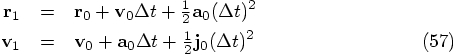
Bob: I guess your lessons were starting to sink in. In any case, let me
put my equations where my mouth is, and let show the idea first for a
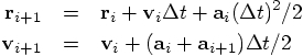
second-order multi-step scheme, a two-step scheme in fact. We start with
the orbit part, where we expand the acceleration in a Taylor series with
just one extra term:
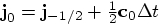
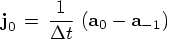
Bob: Speak for yourself, my friends are not jerks. We can determine
the jerk at the beginning of our new time step if we can remember the
value of the acceleration at the beginning of the previous time step, at
time
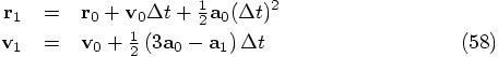
A more direct, but less easily understandable way of writing these
equations is to substitute Eq. (55) into Eq. (57),
in order to get an equation written purely in terms of the accelerations
at different times:
Alice: That is an interesting twist, and indeed a very different approach.
Bob: I have implemented this, starting from the file yo8body.rb,
and renaming it ms2body.rb. I had to make one modification, though.
Previously, we kept track of the number of time steps with a counter nsteps
that was a local variable within the method evolve, but now we need that
information within the multi-step integrator, which I called ms2.
Alice: Why's that?
Bob: A multi-step method is not self-starting, since at the beginning of
the integration, there is no information about previous steps, simply because
there are no previous steps. I solve this by borrowing another 2nd-order
method, rk2 for the first time step. But this means that ms2
has to know whether we are at the beginning of the integration or not, and
the easiest way to get that information there is to make the number of time
steps into an instance variable within the Body class.
What I did was replace nsteps by @nsteps, in the two places
where it was used within the method evolve. I made the same change in the
method write_diagnostics, which simplified matters, since before
we needed to pass nsteps as an argument to that method, and
now this is no longer necessary.
Here is the code:
Alice: So the variable @prev_acc serves as your memory, to store
the previous acceleration. At the start, when @nsteps is still
zero, you initialize @prev_acc, and during each next step, you
update that variable at the end, so that it always contains the value
of the acceleration at the start of the previous step.
Bob: Yes. The acceleration at the end of the previous step would
be the same as the acceleration at the start of the current step, and
that value is stored in the local variable old_acc, as you can
see. This allows me to calculate the jerk.
Alice: Or more precisely, the product of jerk
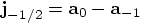
Bob: When I first wrote this, I was wondering whether it was correct
to use this expression for the jerk, since strictly speaking, it gives
an approximation for the value of the jerk that is most accurate at a
time that is half a time step in the past, before the beginning of the
current time step:
But then I realized that the difference does not matter, for a second
order integration scheme. In terms of the next time derivative of
position, the snap
All this would do is to add a term of order
Alice: Yes, from the point of view of a second-order integrator,
the jerk is simply constant, and we can evaluate it at whatever
point in time we want.
Bob: And before I forget, there is one more change I made,
in the file vector.rb, where I gave an extra method to our
Vector class:
Alice: Ah, yes, we only had addition and multiplication methods
before, but when you compute the jerk in ms2 it is most
natural to use subtraction.
Bob: And for good measure, I added a division method as well.
Note that raise is a standard way for Ruby to report an error
condition. Here it is:
Alice: I'm sure that will come in handy sooner or later.
Bob: Let me show that the two-step integration method works.
I'll start again with a fourth-order Runge-Kutta result, as a
check:
Alice: You have been talking about multi-step algorithms.
How does this relate to predictor-corrector methods?
Bob: It is the predictor part of a predictor-corrector scheme.
It is possible to squeeze some extra accuracy out of a multi-step
scheme, by using the information that you get at the end of a step,
to redo the last step a bit more accurately, `correcting' the step
you have just `predicted.'
In this procedure, you do not increase the order of the integration
scheme. So you only decrease the coefficient of the error, not its
dependence on time step length. Still, if the coefficient is
sufficiently smaller, it may well be worthwhile to add a correction
step, in order to get this extra accuracy.
If you would like to know how these methods have been used historically,
you can read Sverre Aarseth's 2003 book Gravitational N-Body
Simulations. He implemented a predictor-corrector scheme in the
early sixties, and his algorithm became the standard integration scheme
for collisional N-body calculations, during three decades. It was only
with the invention of the Hermite scheme, by Jun makino, in the early
nineties, that an alternative was offered.
Alice: I'd like to see a Hermite scheme implementation, too, in that
case. As for the older scheme, is there an intuitive reason that the
corrector step would add more accuracy?
Bob: The key idea is that the predictor step involves an extrapolation,
while the corrector step involves an interpolation. For the predictor
step, we are moving forwards, starting from the information at times
Alice: I see. So the main point is that extrapolation
is inherently less accurate, for the same distance, as interpolation.
Bob: Exactly.
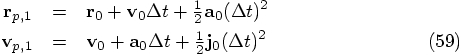
Alice: Let me see whether I really got the idea, by writing it out
in equations. The predicted position
Of course, going back one step will not return us to the same position
but just shifted by one unit in time. Note that our last step has
really been an interpolation step, since we are now using the
acceleration and jerk values at both ends of the step. In contrast,
during the extrapolation step, we used information based on the last
two accelerations, both of which are gained at the past side of that
step.
Bob: Yes, it is nice to show that so explicitly.
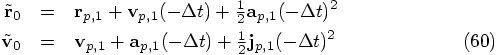
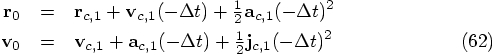
Alice: Now let us engage in some wishful thinking.
We start with Eq. (60) which tells us that we return to the
wrong starting point when we go backward in time. Wouldn't it be
nice if we somehow could find out at which point we should start so
that we would be able to go backwards in time and return to the right
spot? Let us call these alternative position and velocity at time
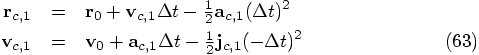
Let us start with the second line in Eq. (63), since that
only involves quantities that are freshly recomputed, namely the
acceleration and jerk, reserving the first equation for later, since
that has a velocity term in the right-hand side. As a first step in
our iteration process, we will simply replace the corrected values on
the right-hand side by the predicted values:
Alice: Well, shouldn't we implement this, too?
Bob: We may as well. It shouldn't be hard.
Alice: So? You look puzzled, still staring at the last set of equations.
Something wrong?
Bob: I'm bothered by something. They just look too familiar.
Alice: What do you mean?
Bob: I've seen these before. You know what? I bet these are just
one way to express the leapfrog algorithm!
Alice: The leapfrog? Do you think we have reinvented the leapfrog
algorithm in such a circuitous way?
Bob: I bet we just did.
Alice: It's not that implausible, actually: there are only so many
ways in which to write second-order algorithms. As soon as you go
to fourth order and higher, there are many more possibilities, but
for second order you can expect some degeneracies to occur.
Bob: But before philosophizing further, let me see whether my hunch
is actually correct. First I'll get rid of the predicted value for
the jerk, using Eq. (61) in order to turn Eq. (68) into
expressions only in terms of the acceleration:
Alice: I guess your friendship with the frog is stronger than mine.
Can you show it to me more explicitly?
Bob: So that you can kiss the frog?
Alice: I'd rather not take my chances; I prefer to let it leap.
Bob: If you plug the expression for
Bob: Yes, apart from one very small detail: if we were to write a
corrected version of ms2, then the very first step would
still have to be a Runge-Kutta step, using rk2. From there
on, we would exactly follow the same scheme as the leapfrog method.
But I agree, no need to implement that.
Alice: And guess what, we got a bonus, in addition!
Bob: A bonus?
Alice: Yes, there is no need for higher iterations, since we have
exactly
Bob: Right you are, how nice! And I'm afraid this is just a fluke
for the second-order case.
Alice: Yes, something tells me that we won't be so lucky when we
go to higher order. 8.1. A Matter of Memory

 .
.
 , as follows:


8.2. Implementation
 and time step
  , in the form of
  ,
since it is only that combination that appears in Eq. (57), which
you write in the next two lines of code. Okay, that is all clear!
,
since it is only that combination that appears in Eq. (57), which
you write in the next two lines of code. Okay, that is all clear!
 , the leading term of the
difference would be:
, the leading term of the
difference would be:
 to the last line in Eq. (57), beyond the purview of a second-order
scheme.
to the last line in Eq. (57), beyond the purview of a second-order
scheme.
   def -(a)
     diff = Vector.new
     self.each_index{|k| diff[k] = self[k]-a[k]}
     diff
   end
8.3. Testing
 |gravity> ruby integrator_driver2j.rb < euler.in
 dt = 0.01
 dt_dia = 0.1
 dt_out = 0.1
 dt_end = 0.1
 method = rk4
 at time t = 0, after 0 steps :
   E_kin = 0.125 , E_pot =  -1 , E_tot = -0.875
              E_tot - E_init = 0
   (E_tot - E_init) / E_init =-0
 at time t = 0.1, after 10 steps :
   E_kin = 0.129 , E_pot =  -1 , E_tot = -0.875
              E_tot - E_init = 1.79e-12
   (E_tot - E_init) / E_init =-2.04e-12
   1.0000000000000000e+00
   9.9499478009063858e-01  4.9916426216739009e-02
  -1.0020902861389222e-01  4.9748796005932194e-01
Here is what the two-step method gives us:
 |gravity> ruby integrator_driver4a.rb < euler.in
 dt = 0.01
 dt_dia = 0.1
 dt_out = 0.1
 dt_end = 0.1
 method = ms2
 at time t = 0, after 0 steps :
   E_kin = 0.125 , E_pot =  -1 , E_tot = -0.875
              E_tot - E_init = 0
   (E_tot - E_init) / E_init =-0
 at time t = 0.1, after 10 steps :
   E_kin = 0.129 , E_pot =  -1 , E_tot = -0.875
              E_tot - E_init = 9.98e-08
   (E_tot - E_init) / E_init =-1.14e-07
   1.0000000000000000e+00
   9.9499509568711564e-01  4.9917279823914654e-02
  -1.0020396747499755e-01  4.9748845505609013e-01
Less accurate, but hey, it is only a second-order scheme, or so we hope.
Let's check:
 |gravity> ruby integrator_driver4b.rb < euler.in
 dt = 0.001
 dt_dia = 0.1
 dt_out = 0.1
 dt_end = 0.1
 method = ms2
 at time t = 0, after 0 steps :
   E_kin = 0.125 , E_pot =  -1 , E_tot = -0.875
              E_tot - E_init = 0
   (E_tot - E_init) / E_init =-0
 at time t = 0.1, after 100 steps :
   E_kin = 0.129 , E_pot =  -1 , E_tot = -0.875
              E_tot - E_init = 1.57e-09
   (E_tot - E_init) / E_init =-1.79e-09
   1.0000000000000000e+00
   9.9499478370909766e-01  4.9916434810162169e-02
  -1.0020897588268213e-01  4.9748796564271547e-01
Alice: It looks like 2nd order, but can you decrease the time step
by another factor of ten?
 |gravity> ruby integrator_driver4c.rb < euler.in
 dt = 0.0001
 dt_dia = 0.1
 dt_out = 0.1
 dt_end = 0.1
 method = ms2
 at time t = 0, after 0 steps :
   E_kin = 0.125 , E_pot =  -1 , E_tot = -0.875
              E_tot - E_init = 0
   (E_tot - E_init) / E_init =-0
 at time t = 0.1, after 1000 steps :
   E_kin = 0.129 , E_pot =  -1 , E_tot = -0.875
              E_tot - E_init = 1.63e-11
   (E_tot - E_init) / E_init =-1.86e-11
   1.0000000000000000e+00
   9.9499478012623654e-01  4.9916426302151512e-02
  -1.0020902807186732e-01  4.9748796011702123e-01
Bob: This makes it pretty clear: it is a second-order scheme.
8.4. Stepping Back
 and
and  , to estimate the situation
at time
, to estimate the situation
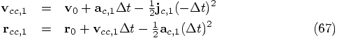
at time  . For the corrector step, effectively
what we do is to go back in time, from
. For the corrector step, effectively
what we do is to go back in time, from  back to
 . Of course, we don't get precisely back to the same
position and velocity that we had before, so the difference between
the old and the new values is used to correct instead the position and
velocity at time
. Of course, we don't get precisely back to the same
position and velocity that we had before, so the difference between
the old and the new values is used to correct instead the position and
velocity at time  .
.
 and
velocity
and
velocity  are determined as follows:
 using these new values for the position
and the velocity, we can take a step backwards.
using these new values for the position
and the velocity, we can take a step backwards.
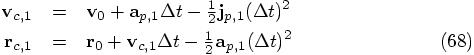
 and velocity
  that we started with.
Instead, we will obtain slightly different values
that we started with.
Instead, we will obtain slightly different values
 and
and  for the position
and velocity at time
for the position
and velocity at time  , as follows:
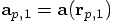 and where
  is the jerk obtained now from the last two values of the acceleration:

8.5. Wishful Thinking.
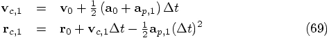
 the corrected values:
  for
the position and
for
the position and  for the velocity. If our wish
would be granted, and someone would hand us those values, then they
would by definition obey the equations:
for the velocity. If our wish
would be granted, and someone would hand us those values, then they
would by definition obey the equations:
 and
and  is the jerk that would be obtained from the
last two values of the acceleration, including the as yet unknown
corrected one:
is the jerk that would be obtained from the
last two values of the acceleration, including the as yet unknown
corrected one:


 and
and  , we can obtain
those as:
, we can obtain
those as:
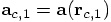
8.6. An Old Friend
 in the
first line of Eq. (69) back into the right-hand side of the
second line, you get:
in the
first line of Eq. (69) back into the right-hand side of the
second line, you get:
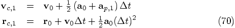
 and
and
 . This is because the leapfrog is
time reversible as we have shown before.
. This is because the leapfrog is
time reversible as we have shown before.