3.3 Running a Code

Carol:

That's it, the last bug caught, our forward_euler1 compiled at last! Let's see what it produces. Since we asked for the output of positions and velocities for 10 time units at intervals dt = 0.01, our screen will be flooded by 1000 lines of output; better to redirect the output to a file. Let's call it forward.out, and let's have a look at the beginning and the end of the file, say five lines each:

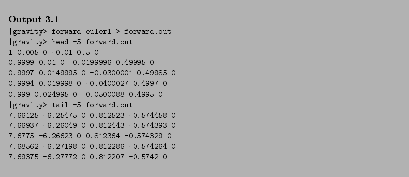
Bob:

Hey, Alice told us that our two particles were at apocenter initially, at distance 1, which meant that they could come closer but that they would never get further away from each other than unity in our length units. And here we have distance vectors larger than 7, actually close to 10 if I remember my Pythagoras formula well enough, in the last line.

Carol:

You are right, slightly more than 9.9:

|gravity> bc
7.69375*7.69375 + 6.27772*6.27772
98.6035574609
sqrt(98.6035574609)
9.92993239961380603154
|gravity>

Bob:

Unix takes a while to get used to! What does the two-letter `word' bc mean?

Carol:

Oh, bc is a more powerful version of dc, which stands for `desk calculator' and is a simple utility to quickly find arithmetic answers without writing a program. Here is what the manual page for dc tells us:

|gravity> man dc
NAME
     dc - desk calculator

SYNOPSIS
     dc  [ filename ]

DESCRIPTION
     dc  is an arbitrary  precision  arithmetic  package.   Ordi-
     narily  it operates on decimal integers, but one may specify
     an input base, output  base,  and  a  number  of  fractional
     digits  to  be maintained. The overall structure of dc  is a
     stacking (reverse Polish) calculator.   If  an  argument  is
     given,  input  is  taken  from that file until its end, then
     from the standard input.

     bc  is a preprocessor for dc  that provides  infix  notation
     and  a  C-like  syntax  that implements functions.  bc  also
     provides reasonable control  structures  for  programs.  See
     bc(1).
|gravity>

Carol:

With dc we could not have used the sqrt() function, so we used bc; perhaps it stands for a `better calculator', who knows.

Bob:

Well, our program compiles and our program runs, so we have passed two barriers, but now it gives answers that are not sensible. The third step that could have gone wrong is that we have somehow made a mistake in our algorithm, mistyping it, or even being misguided as to its structure. But with the simplicity of Eqs. 3.1, 3.2 it seems clear that neither is the case here. The equations tell the particle to `follow its nose' in a straight line during each time step. What could be simpler!

Alice:

You are right. After syntactic compile time errors, dynamic run time errors, and semantic errors in coding up the algorithm correctly, the fourth potential source of errors lies in using the algorithm. While it seems that we took an almost ridiculously small time step, the choice dt = 0.01 may still be too large. After all, dt is the only free parameter in our program. The code is like a laboratory instrument, a black box with only one dial, so we may as well play with different settings of the dial.

Bob:

Indeed, we had no particular reason to choose the value we did, rather than any other. But before we start playing, can we plot a picture of the orbit we just computed? I'd rather have a real sense of what is going on, beyond staring at a few output numbers.

Carol:

Will do, but may I add another option to Alice's detective analysis? Apart from the four types of error that she mentioned, there is another possibility. We are not really sure that the program we ran was the one we wrote. The default search path on this computer may be set such that we wind up invoking another program with the same name.

Bob:

Also called forward_euler1? That seems extremely unlikely!

Carol:

But as they say in the Hitchhiker's guide to the galaxy, not impossible. Let me try, and force execution from the current directory ``.'' by adding it to the name of our executable:

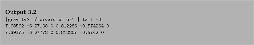
Carol:

Okay, no problem here. I just thought I'd bring up something I happened to learn in class today. Now let's look at a picture of the orbit. I suggest using gnuplot, present on any Linux running system, and something that can be easily installed on many other Unix systems as well. To use it is quite simple, with only one command needed to plot a graph. In our case, however, I'll start with the command set size ratio -1. A positive value for the size ratio scales the aspect ratio of the vertical and horizontal edge of the box in which a figure appears. However, in our case we want to set the scales so that the unit has the same length on both the x and y axes. Gnuplot can be instructed to do so by specifying the ratio to be -1. In fact, let me write the line set size ratio -1 in a file called .gnuplot in my home directory. That way we don't have to type it each time we use gnuplot. Okay, done. Now let's have our picture:

|gravity> gnuplot
gnuplot> set size ratio -1
gnuplot> plot "forward.out"
gnuplot> quit
|gravity>

Figure 3.1: Relative orbit for the first attempt to integrate a two-body system with a forward-Euler integrator, with time step $dt = 0.01$

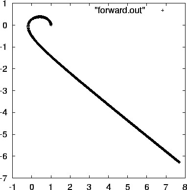Bob:

Wow, the two stars were flung away as by a slingshot, after only slightly more than half an orbit. I guess that indeed the time step was too large.

Alice:

I think you are right. Notice that the artificial slingshot, caused by numerical errors, occurred just after pericenter, where the curvature of the orbit is highest. Stepping along tangentially to the orbit tends to let you spiral out from the original orbit, and this effect is higher when the orbital curvature is higher.

Carol:

Okay, I'll change the time step size.