3.6 Finding (slow) Convergence

Alice:

Ready for a ten times smaller time step?

Carol:

We aim to please!

Bob:

Somewhat better, but still the separation vector has a length greater than unity, which is not physical. Let's look at a picture. I saw that you wrote this line set size ratio -1 in .gnuplot, so I guess you only have to issue the plot command.

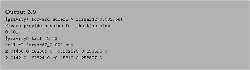
|gravity> gnuplot
gnuplot> plot "forward2_0.001.out"
gnuplot> quit
|gravity>

Figure 3.2: Relative orbit for the second attempt to integrate a two-body system with a forward-Euler integrator, with time step $dt = 0.001$

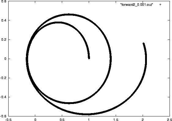Alice:

At least we got two revolutions this time.

Carol:

Let's try a couple more steps of ten refinement of the step size. But before we do that, let us be a bit more frugal in our output. I just noticed that our output files are growing alarmingly in size:

|gravity> ls -l *.out
-rw-r--r--    1 carol    students    39633 Dec 24 07:07 forward1.out
-rw-r--r--    1 carol    students   404204 Dec 24 11:27 forward2_0.001.out
-rw-r--r--    1 carol    students    39673 Dec 24 10:31 forward2_0.01.out
|gravity>

Bob:

I see! Our last file had a size of 400 kbytes, which is not much of a problem. But with two more steps of refinement we would wind up with a 40 Mbyte file. Even though our disk space is large enough, it would surely slow down both gnuplot and postscript plotting. How about restricting output to occur only once every dt_out = 0.01, even if our time step dt < dt_out?

Carol:

That's what I had in mind. Time for a new version:

Carol:

As before, let us first look at the end of the output file, to see whether the numbers at least look reasonable.

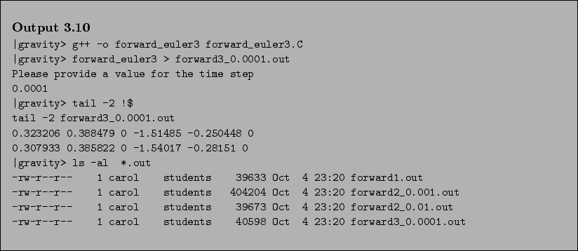
Bob:

Ah, for the first time the separation vector is consistent, at least in principle, since now it is shorter than unity.

Carol:

And the output size is under control now. Time to make a plot, but I'm getting a little tired of the label written in the top right hand corner with the one lonely plot symbol. I'll add the notitle command.

|gravity> gnuplot
gnuplot> plot "forward3_0.0001.out" notitle
gnuplot> quit
|gravity>

Figure 3.3: Relative orbit for the third attempt to integrate a two-body system with a forward-Euler integrator, with time step $dt = 0.0001$

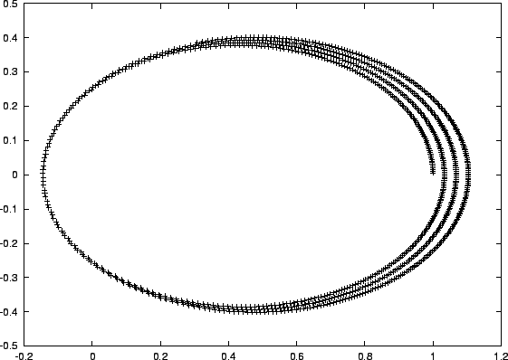Carol:

Three revolutions and counting! And there does seem to be a definite convergence toward an ellipse, which is encouraging. Okay, ready for another shrinking by ten of the time step?

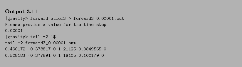
Bob:

We are finally beginning to give the computer a workout, with our request to take a million steps! But note that we are still not converging very quickly. The numbers are once more quite different from what we saw when we took `only' a hundred thousand steps!

|gravity> gnuplot
gnuplot> plot "forward3_0.00001.out" notitle
gnuplot> quit
|gravity>

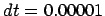
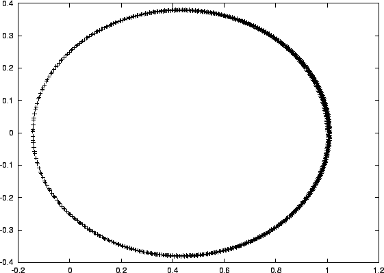Figure 3.4: Relative orbit for the fourth attempt to integrate a two-body system with a forward-Euler integrator, with time step $dt = 0.00001$

Carol:

But this time the orbit looks almost natural. I bet that with another refinement of the step size by a factor ten, we would finally see convergence.

Bob:

Disappointing, I must say. At least we got the first decimal right, more or less, but that's about it. Let's see whether the figure finally looks like an honest ellipse.

|gravity> gnuplot
gnuplot> plot "forward3_0.000001.out" notitle
gnuplot> quit
|gravity>

Figure 3.5: Relative orbit for the fifth attempt to integrate a two-body system with a forward-Euler integrator, with time step 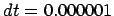$dt = 0.000001$

Alice:

That looks more like it. Interesting, by the way, to see the speed up of the relative motion of the two particles near pericenter, in the last three figures: you can see that from the wider spacing of the particles, something that was lost when we went to a higher density of output points.

Carol:

Let's do one more step of ten refinement in step size. Modern computers should not have much trouble taking a hundred million time steps, after all. And since the plot will not change much any more, let us directly look at the last lines of the output:

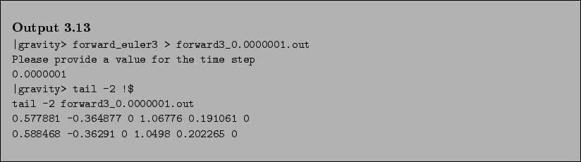
Carol:

There you go, Bob, convergence to two significant digits at least! Even so, I guess we are all convinced that first-order methods are not the way to go. Time to go to second order!

Alice:

So let's write a leapfrog code. But before doing so, there is still one addition I would like to make to our poorly performing forward Euler code. You see, for the two-body problem we can get a pretty good idea of what's going on by looking at the orbit, because we know what to expect. In fact, we can solve the orbit analytically, and therefore we can compute everything to arbitrary accuracy that way, much faster and cheaper than doing it the hard way, through numerical orbit integration. The point is that for an $N$-body system with $N>2$ the orbits don't look recognizable at all, and we would be hard put to judge the performance of a code from staring at orbital figures.

Bob:

Ah, you mean that we should try to define, what did they call it in physics class, conserved quantities?

Alice:

Exactly. And the simplest such quantity is the total energy of the $N$-body system. We know that it is rigorously conserved, so any deviation between beginning and end of a numerical integration session must be purely the result of numerical errors.

Carol:

Okay, let's code that up too, and then call it a day. What are the equations?