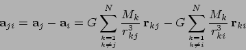
The most symmetric Hermite version, and the one closest resembling the leapfrog is this one:
Here
![]() is the jerk, the time derivative of the
acceleration, and therefore the third time derivative of position:
is the jerk, the time derivative of the
acceleration, and therefore the third time derivative of position:
| (6.3) |
The term `jerk' has crept into the literature relatively recently, probably originally as a pun. If a car or train changes acceleration relatively quickly you experience not a smoothly accelerating or decelerating motion, but instead a rather `jerky' one.
The jerk can be computed through straightforward differentiation of Newton's gravitational equations, Eq. 5.2:
where
![]() .
.
As an aside, note that the jerk has one very convenient property.
Although the expression above looks quite a bit more complicated than
Newton's original equations, they can still be evaluated through one
pass over the whole ![]() -body system. This is no longer true for
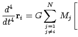
higher derivatives. For example, we can obtain the fourth derivative
of the position of particle
-body system. This is no longer true for
higher derivatives. For example, we can obtain the fourth derivative
of the position of particle ![]() (the snap, see next section) by
differentiating Eq. 6.4:
(the snap, see next section) by
differentiating Eq. 6.4:
where
![]() , and this is the expression that
thickens the plot. Unlike the
, and this is the expression that
thickens the plot. Unlike the ![]() and
and ![]() expressions,
that are given by the initial conditions,
expressions,
that are given by the initial conditions, ![]() has to be
calculated from the positions and velocities. However, this
calculation does not only involve the pairwise attraction of particle
has to be
calculated from the positions and velocities. However, this
calculation does not only involve the pairwise attraction of particle
![]() on particle
on particle ![]() , but in fact all pairwise attractions of all
particles on each other! This follows immediately when we write out
what the shorthand implies:
, but in fact all pairwise attractions of all
particles on each other! This follows immediately when we write out
what the shorthand implies:
 |
(6.6) |
When we substitute this back into Eq. 6.5, we see that
we have to do a double pass over the ![]() -body system, summing over
both indices
-body system, summing over
both indices ![]() and
and ![]() in order to compute a single fourth derivative
for the position of particle
in order to compute a single fourth derivative
for the position of particle ![]() .
.
![\begin{displaymath}
{\bf j}_i = G \sum_{j=1 \atop j \neq i}^N \,M_j \left[
\frac...
...({\bf r}_{ji}\cdot{\bf v}_{ji}){\bf r}_{ji}}{r_{ji}^5}
\right]
\end{displaymath}](img489.png)
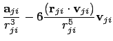
![$\displaystyle + \left\{ -3\frac{v_{ji}^2}{r_{ji}^5}
-3 \frac{({\bf r}_{ji}\cdot...
...c{({\bf r}_{ji}\cdot{\bf v}_{ji})^2}{r_{ji}^7} \right\} {\bf r}_{ji} \,\,\Bigg]$](img497.png)