9.3 Testing, testing, . . .

Bob:

Short and sweet, as they say. But perhaps a bit too short, especially on explaining how exactly we managed to put particles in a sphere using a, what did you call it, spherical coordinate system?

Alice:

Yes, that is a coordinate system that is a lot more convenient for dealing with spheres than the usual Cartesian coordinate system is; the latter would of course be better if we were to build a star cluster with the shape of a box.

Bob:

I'd prefer the shape of a diamond over that of a box. But seriously, how I am to know for sure that the equations you gave me from your physics course are actually correct?

Carol:

The answer they keep repeating in my courses: testing, testing, ...

Bob:

Okay, let's just run the program with a few particles, okay? By just looking at the numbers we may get an idea of whether we are at least approximately right. Alice, you're at the keyboard. Have a go at it!

Alice:

Fine. How about ten particles?

|gravity> sphere1a -n 10
seed = 1063894860
10
0
0.1 0.4540028492193794 0.3498769522044687 0.7969703663542103 0 0 0
0.1 0.03987844095394553 -0.08119205595973951 -0.6615273048865606 0 0 0
0.1 -0.07696021131813481 -0.8459387776849843 0.3519731575017572 0 0 0
0.1 -0.03159529410632059 -0.2076818100526642 0.7862706899063225 0 0 0
0.1 0.02919115871639223 -0.228846199565124 0.2176806328285098 0 0 0
0.1 0.531084745743273 -0.1003377930427043 -0.05342966914946958 0 0 0
0.1 0.7662014881610754 -0.3620973663404717 0.1670139579482853 0 0 0
0.1 0.2522400702554067 -0.6696003994776 -0.08285809759917392 0 0 0
0.1 0.2785462467572272 0.06099199162060588 0.536196594372378 0 0 0
0.1 -0.510335018159465 0.06233465247130211 0.7635335045998497 0 0 0
|gravity>

Bob:

At least the velocities are zero, and the position coordinates are smaller than one.

Carol:

And larger than minus one. So far so good.

Alice:

Not only that, if one of the numbers comes close to one in absolute value, the other numbers are smaller. Indeed, it seems that the sum of the squares of the position coordinates is always smaller than unity, as it should be: the particles neatly lie in a sphere.

Bob:

But do they lie homogeneously in a sphere?

Carol:

I see large and small numbers, positive and negative numbers, so that all suggest that things are pretty random.

Alice:

Bob is right, we really should check for homogeneity. Random is not enough, since a random distribution could still be skewed one way or other.

Bob:

How do you test a sphere for homogeneity?

Carol:

I've done some video game programming, where the hardest part was always to get the 3D aspects right, especially rotations. They even had us learn about quaternions!

Bob:

quarter whats?

Carol:

Quaternions. Four-dimensional numbers, analogies of complex numbers, that are two-dimensional when expressed in terms of real components. Really neat stuff.

Bob:

For now, let's keep it simple. How about just making a picture of it? It would be a two-dimensional projection, but if the three-dimensional distribution would be wildly inhomogeneous, you would think that it would show up even in projection.

Alice:

Good idea. Let us use our gnuplot once more. But now we have to rethink how to get our data into the gnuplot program. In the past, we just took the output file, since the first two numbers on each line happened to be the $x$ and $y$ coordinates. But with our new fancy integrator, the first two lines contain the number of particles and the time, respectively, and then each line contains first the mass, and only then positions and velocities.

Carol:

This is a good use for the tail command in unix.

Bob:

Aren't we interested to modify the head part of the file, rather than the tail? I thought tail -20, for example, gives you only the last 20 lines of a file.

Carol:

True, but there is a + option as well. If you type tail +3, you get the whole file, but starting at the third line, in other words skipping the first two lines; all the rest is than the `tail' of the file.

Alice:

So we will run our sphere1a code and then pipe the results into tail:

|gravity> sphere1a -n 10000 | tail +3 > test1a_10000.out
seed = 1063986021
|gravity> head -3 !$
head -3 test1a_10000.out
0.0001 0.5710408801016649 -0.3784997794699326 0.1014650450926402 0 0 0
0.0001 0.9204463477655462 0.1904132590373278 -0.1316466915348289 0 0 0
0.0001 -0.06164472062611391 0.1087990388945161 0.7259008589013708 0 0 0
|gravity> tail -3 test1a_10000.out
0.0001 0.01308756829247314 -0.06368169834698917 0.7647793506402052 0 0 0
0.0001 0.001461596716547156 0.1127385579637729 0.6880562520087973 0 0 0
0.0001 0.05993388699838697 -0.3903340594881157 0.6016407318791096 0 0 0
|gravity> wc !$
wc test1a_10000.out
  10000   70000  718902 test1a_10000.out
|gravity>

Bob:

Good! Indeed there are ten thousand lines, and the first few and last few lines all have the right form. So we must be doing something right!

Alice:

Now let us see how to get gnuplot to show the data from the second and third column, the $x$ and $y$ components of the positions.

|gravity> gnuplot
Terminal type set to 'x11'
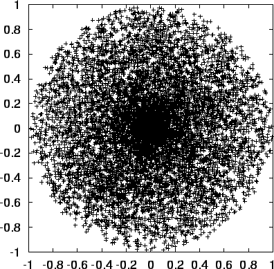
gnuplot> plot "test1a_10000.out" using 2:3 notitle
gnuplot>

Figure: Output of sphere1a, with 10,000 particles, projected onto the $\{x,y\}$ plane

Carol:

(fig. 9.1) Looks good to me. The particles are closer together in the center than near the edge, but that must be because we see more volume there, when we project the sphere on a two-dimensional screen.

Alice:

Yes, near the edge your line of sight only intersect a small sliver of the sphere. Although the density is homogeneous, that still gives you only a few particles.

Bob:

I guess we all believe our sphere.C program to be correct now, but just to make sure, let us plot another view, now that we have an easy way to do that.

Carol:

You are hard to satisfy! But sure, why not. Let take the $x$ and $z$ components of the positions, this time.

Alice:

Okay, this is how to produce that picture:

|gravity> gnuplot
Terminal type set to 'x11'
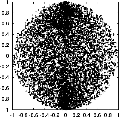
gnuplot> plot "test1a_10000.out" using 2:4 notitle
gnuplot>

Figure: Output of sphere1a, with 10,000 particles, projected onto the $\{x,z\}$ plane

Carol:

(fig. 9.2) Wow! That's weird! What are those extra particles doing there, along the vertical line in the middle of the picture? That doesn't look at all like a projection of a homogeneous sphere.

Bob:

(smiling) So much for chiding me about testing too much.

Carol:

Well, I must say, I'm glad now that you were hard to satisfy. If you wouldn't have insisted we would have moved right along. Who knows how long it would have taken us to find that bug, whatever it is ...

Alice:

...if we had ever found it. This is something scare about using computers: you know you have done something wrong, when you see that things don't look right, but the other way around does not hold. Things can look pretty right all right, and still be wrong.

Bob:

That reminds me of a philosopher, was it Popper, who said that you can never verify a theory. You can only falsify it.

Carol:

Yes, that was him. The best you can do is to make a theory more and more plausible. And yes, the same holds true for programming. There is a whole branch of computer science that deals with proving the correctness of code. However, they only talk about the internal correctness of a code. And that's the only thing they can possibly talk about, since no compiler can ever test whether or not the external information has been put in correctly. If the physics input is wrong, there is no logical way for any software program to find that out.

Bob:

True, although here we are really working with math more than physics, assigning points to positions in space. But I see your point. Still, physics is presumably consistent, so even there one can apply consistency checks.

Carol:

Yes, in a large system you must be right, but I'm not sure how far you can get with such a small code as sphere.C. It's a bit embarrassing, frankly, to get such a wrong result with so few lines of code.

Alice:

Oh, believe me, I've made bigger mistakes in smaller codes. But let's put the philosophy aside for now, and let's fix things! But first I want to know precisely what's going on. Let's take somewhat fewer particles, and let us look at both picture again, just to have another way of approach this mystery.

Carol:

Here you are, with a thousand particles, instead of ten thousand. First the $x$ and $y$ components of the positions.

|gravity> sphere1a -n 1000 | tail +3 > test1a_1000.out
seed = 1063987133
|gravity> gnuplot
Terminal type set to 'x11'
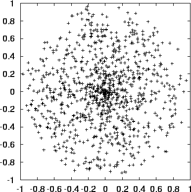
gnuplot> plot "test1a_1000.out" using 2:3 notitle
gnuplot>

Figure: Output of sphere1a, with 1,000 particles, projected onto the $\{x,y\}$ plane

Bob:

(fig. 9.3) Now this looks okay again, as before. However, I must say, I'm a little puzzled by the fact that there are so many particles in the center. To have the density petering off toward the edge seems reasonable, as we discussed a little earlier. But why should there be a spike in particle density near the center?

Carol:

Good question. Let's first look at the $\{x,z\}$ view.

|gravity> gnuplot
Terminal type set to 'x11'
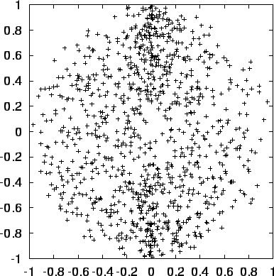
gnuplot> plot "test1a_1000.out" using 2:4 notitle
gnuplot>

Figure: Output of sphere1a, with 1,000 particles, projected onto the $\{x,z\}$ plane

Carol:

(fig. 9.4) Same problem: too many particles near the central vertical.

Bob:

Aha! Now I can answer my own question. Of course! If there are really too many particles near the central vertical line in the $\{x,z\}$ plane, then that excess of particles will all be projected near the center of the $\{x,y\}$ projection.

Alice:

Good point indeed! At least the bug we have found is consistent. I am glad we are dealing with only one problem, rather than too!

Carol:

But I would prefer to have no bug at all. Let's have another look at the code.