9.4 Chasing the Bug

Bob:

Well, the one part which I must admit I did not fully understand is where the angles are used to create particle positions in, what did you call it again?

Alice:

spherical coordinates. A useful way to label particles by their distance from the center, and by the two angles needed in addition to locate them uniquely.

Carol:

Useful, yes, if they do what they are supposed to do. Bob may be right, that is a likely place to have made a mistake. Let us look at how exactly we made that transformation. Here is how we assigned the positions and velocities to all the particles.

Alice:

At first sight, it looks rather reasonable. I clearly recognize the spherical coordinate angles in the position assignments: the sines and cosines of $\theta$ and $\phi$ are all in the right place.

Carol:

And the ranges above those three lines are correct too: $\theta$ moves from the north pole to the south pole, so to speak, which makes an arc of $180^o$, starting at $\theta = 0$, as it should; similarly $\phi$ moves all the way around along the equator, describing an angle of $360^o$. What could possibly be wrong?

Bob:

Why are the $r$ values distributed according to a one-third power?

Alice:

That's because the size of a volume element increases with the cube of $r$. For example, if you double the radius of a three-dimensional object, you make the volume eight times large. In order to keep the same density of points, you have to put eight times as many particles.

Bob:

I see. You want to distribute the particles uniformly random in $r^3$, not in $r$. So this means that $r$, which is the third root of $r^3$, has to follow the third root of a uniformly distributed variable.

Alice:

You got it.

Bob:

And the angles don't need such a trick, because $r$ does not change while we move around the latitude $\theta$ or the longitude $\phi$.

Alice:

Right you are, that is indeed ...OOPS ...no ...correction ... that is not indeed right, that is wrong. Now I see our mistake!

Carol:

But look, if you go around the equator, how can it make any difference to where on the equator you are?

Alice:

It doesn't, but try going to one of the poles.

Carol:

Ah, now I get it. Moving from the equator to the pole, the lines of constant longitude converge together, and there is less and less room between them, the closer you get to the pole.

Alice:

And mathematically you express that by the expression for a volume element $dV$ as:

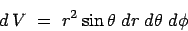$$d\:V \; = \; r^2 \sin \theta \; dr \; d\theta \; d\phi$$ (9.1)

Alice:

And for our application, it is easier to write this as

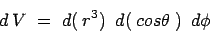$$d\:V \; = \; d(\: r^3)\: \; d(\: cos \theta \:)\: \; d\phi$$ (9.2)

Bob:

So this means that we have to invert the cosine factor for $\theta$, just as we inverted the third power for $r$ in the line above in our code.

Alice:

Exactly. And the inverse of `$\cos \theta$' is ` $\rm {acos}\, \theta$, sometimes also written as ` $\arccos \theta$.' If we sprinkle particles along latitude in such a way that we do it as the arc cosine of $\theta$, we will no longer overpopulate the poles.

Carol:

Ah, so that is what cause the crowding at the poles, something that showed up only in the $\{x,z\}$ plot.

Bob:

Because in the $\{x,y\}$ plot the poles are projected in the middle of the equatorial plane. The bug was less obvious there, although it did create the spike in the center, which we all overlooked in the first figure, which was a bit crowded with $10,000$ particles.

Alice:

Well, I'm really glad we have found the bug, and it is easy to fix. Let us call the corrected code sphere1.C. The only difference is the line for assigning random number values to $\theta$:

|gravity> diff sphere1.C sphere1a.C
197c197
< 	real theta = acos(randinter(-1.0, 1.0));
---
> 	real theta = randinter(0.0, PI);
|gravity> 
\cba

\abc

\carol
Let's see whether things come out better.

\cba

\begin{small}
\begin{verbatim}
|gravity> sphere1 -n 1000 | tail +3 > test1_1000.out
seed = 1063988487
|gravity> gnuplot
Terminal type set to 'x11'
gnuplot> plot "test1_1000.out" using 2:3 notitle
gnuplot>

Figure: Output of sphere1, with 1,000 particles, projected onto the $\{x,y\}$ plane

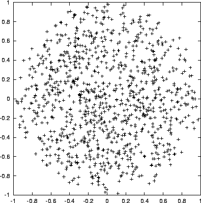Bob:

(fig. 9.5) What a difference a line of code can make! No spike in the center any more. Everything looks so much smoother.

Carol:

Indeed. There is only a mild edge effect, with somewhat fewer particles far away from the center, but the contrast between center and edge is much less than it was before.

Alice:

This suggest that our central vertical line has cleared away. Let's make sure.

|gravity> gnuplot
Terminal type set to 'x11'
gnuplot> plot "test1_1000.out" using 2:4 notitle
gnuplot>

Figure: Output of sphere1, with 1,000 particles, projected onto the $\{x,z\}$ plane

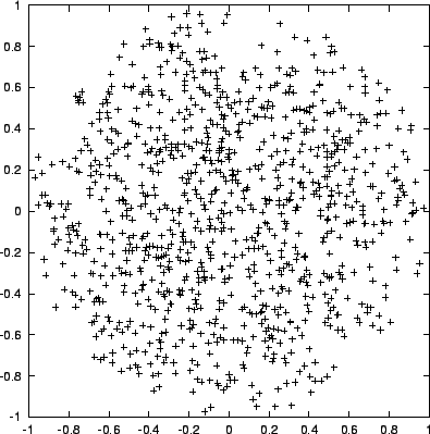Bob:

(fig. 9.6) Indeed, a clean bill of health for sphere1.C

Carol:

The moral of the story seems to be to try to test each module before you start putting things together, no matter how tempting it is to quickly write a few pieces and do some fun experiment with it.

Bob:

Yes, and this must be equally true for real experiments as well as for virtual experiments in cyberspace. This reminds me of what I just heard from a friend of mine, a graduate student in physics. He talked about an experiment he was involved in. The wanted to test a new magnet, to be used to deflect a particle beam, in his case a beam of polarized electrons. After finishing the construction of the magnet setup, they bought a standard device that produced polarized electrons of the right type, hooked it up to the magnet, and switched everything on. If all had gone well, fine, but in their case things did not go well. The result is not what they expected, and they didn't know at that point whether there was something wrong with the magnet, with the gadget producing the electrons, with the connection between the two devices, or with the apparatus reading out the results (or even with the operator of the equipment who might have had a bad day and therefore made some kind of mistake).

Alice:

It would have been worse, much worse actually, if all had seemed fine at first, but only because some subtle bug in one of the devices produced an error that happened to be canceled more or less by another error in another part of the setup.

Bob:

That was his conclusion too. He told me he realized that it is crucially important to test one by one all the steps in constructing an experimental setup. The first step should have been to make sure that the gadget generating the electrons is really doing what they expected and hoped it would do. In other words, they should first have carefully measured the properties of the electron beam before it entered the magnet setup. Only when they really felt comfortable that their gadget was working as advertised would it make sense to connect it to the magnet, and to start analyzing the beam coming out of the magnet.

Carol:

I think the analogy is a good one, and that what is true for a traditional lab is true for our virtual lab as well. We did not really confront this problem earlier, since we dealt only with two or three particles, for which we wrote the initial conditions by hand. In contrast, we now have reached a point where for the first time we are generating initial conditions automatically. And anything that is done automatically can go wrong in all kind of unexpected ways.

Alice:

Well, it is still possible to make mistakes when entering numbers by hand. I sure have done that more often than I'd like to admit.

Carol:

Of course, but when you are dealing with a two-body or three-body system, you can track the orbits individually on the screen, and if you are careful, you will notice if the particles behave completely different from what you expected. But as soon as we start generating initial conditions automatically in large numbers, for a 25-body system for example, the situation is drastically different. It is no longer possible to look at the spaghetti of tangled orbits on a screen and to decide whether all 25 particles do even remotely what they are supposed to do. And indeed, the whole reason to use a computer, rather than pen and paper, is to solve a problem that is too complex to predict analytically beforehand. So you don't know in detail what to expect, and you may not notice if any part of the system behaves differently from how it should behave.

Bob:

I bet your must have heard about modular testing in one of your computer science classes.

Carol:

Yes, but frankly I thought they exaggerated a bit. The typical home work problems were often so simple that it was easy to see whether you got it right or not. But with our example today, I can see how essential it is to test each and every module you write, before hooking it up to other modules. If you test modules one by one, then it is most likely that a new bug in a complex of modules is generated by the latest module you have just added; or at least is caused by an unexpected interaction between that new module and what was already tested before. In both cases, you are far better off than if you suddenly have to test a whole conglomeration of modules, where errors could be hidden in any of them.

Alice:

That last scenario is a nightmare, and a good way to quickly loose interest in computer programming.

Exercise 9.1 (Rejection technique)
Inspect the following code. It uses a completely different technique to generate initial conditions for a homogeneous sphere. It is simpler in that it does not use any trigonometric functions, but only the usual Cartesian coordinates. This sounds almost too good to be true. Can you figure out how the rejection technique works? Try it out and compare its results with that of sphere1.C.